Skip to content

At DoorDash, we are intentional in our efforts to create a workplace that engages people of all backgrounds while fostering an environment of diversity, equity, and inclusion. Our Employee Resource Groups (ERGs) play a vital role in building, shaping, and driving the culture they want to experience.

This February, in collaboration with our Black@ Employee Resource Group, we continue to acknowledge and reflect on the significance of Black history while embracing and embodying this year’s theme of Black Resistance. 

“I connect with the theme of Black Resistance by my mere existence. I’ve traced my family back to 1775, living as enslaved people in Georgia. Generations had to resist so much just for me to exist! Beyond that, I’m existing as a Black woman with multiple STEM degrees working in tech. If that’s not Black Resistance, I don’t know what is.”
L. Patrice Bell, Manager, Strategic Initiatives at DoorDash and Black@ lead

We’re kicking off Black History Month with an exploration of how Black professionals face, navigate, and overcome careers in resistant spaces through a Black Resistance Within Tech panel discussion, including Kofi Amoo-Gottfried, our Chief Marketing Officer; Kaetlin Andrews, our Senior Manager, Regional Partner Strategy; DeVaris Brown, Founder and CEO of Meroxa Data; and Courtnee Futch, Director of Brand Marketing & Partnerships at EatOkra.

Inclusive programming includes a Radical Care Workshop with Heal Haus designed to discuss how stress shows up in the workplace and how we can support one another, a special fireside chat with actors/authors Kirby Howell-Baptiste and Larry Fields III, a coordinated meetup in local office hubs for a Black@ WeDash, a virtual Black History Tour exploring the art, history, and soul of Washington, D.C., and we will wrap up our celebration with a virtual block party featuring a live DJ and appearances from artists and comedians. 

Throughout the year, DoorDash works to empower communities of color through our work to broaden food access, our Accelerator for Local Restaurants and Accelerator for Local Goods, and our Dasher financial empowerment work. Since launching in 2018, almost 80 percent of deliveries powered by Project DASH have gone to communities of color. Our partnership with the National Urban League — the country’s largest and oldest civil rights organization, has also helped over 10,000 Dashers earn, save, and invest through financial empowerment curriculum on GoalUp.org, and supported local communities and Urban League affiliates across the country. Merchants across the U.S. have been able to grow their businesses through the grants and training provided via our merchant empowerment work with 87 percent of restaurant owners participating in the Accelerator For Local Restaurants cohorts identifying as people of color and 40 percent of Accelerator for Local Goods participants identifying as Black or African American.

We will continue to prioritize investing in and advancing opportunities for historically underrepresented people. Our success as a company is firmly rooted in our inclusive culture and in advancing diversity throughout DoorDash to ensure we reflect the global audiences we serve, with learning and development opportunities available to corporate team members covering topics such as how to support allyship, how to speak up against racism at work, and more. 

Our efforts to create a workplace where everyone feels welcomed, supported, and valued is one of the reasons we were recently recognized as one of America’s Greatest Workplaces 2023 by Newsweek. To learn more about this award and how we’ve driven the culture our employees experience over the last year, click here.

It would be almost impossible to build a scalable backend without a scalable datastore. DoorDash’s expansion from food delivery into new verticals like convenience and grocery introduced a number of new business challenges that would need to be supported by our technical stack. This business expansion not only increased the number of integrated merchants dramatically but also exponentially increased the number of menu items, as stores have much larger and more complicated inventories than typical restaurants. This increased volume of items created high latency and high failure rate in the fulfillment backend mainly caused by database scalability problems.

To address these scalability issues we did a major overhaul of the legacy architecture and adopted CockroachDB as its new storage engine. Our team’s goal was to utilize CockroachDB to build a scalable and reliable backend service that could fully support our business. CockroachDB is a scalable, consistently-replicated, transactional datastore, and it’s designed to run on the cloud with high fault tolerance.

This article will take a deep dive into the steps we took to migrate over to CockroachDB and how we ensured that migration was smooth and successful. Specifically we will discuss:

  • The issues and problems associated with the legacy store_items implementation
  • Why we chose CockroachDB
  • How we migrated to CockroachDB successfully
  • Our results and learnings

The challenges with the legacy store_items implementation

store_items is a materialized view that contains catalog, inventory, and pricing data for all the convenience and grocery items. It’s hosted in the PostgreSQL and used to serve item metadata to the Dasher, our name for delivery drivers, during order fulfillment.

Our legacy store_items table had successfully gotten the new vertical business started, but needed to be a lot more scalable if we wanted to support 10x volumes. There were three main concerns that we needed to address: 

  • Performance concerns 
  • Maintenance concerns 
  • Anti-patterns that needed to be fixed

Let’s dive into each one of these:  

Performance concerns:

As our use cases evolved, our OLTP database usage went up to 500GB very quickly, which was problematic as our internal recommended single PostgreSQL table size is under 500GB. Tables over the limit can become unreliable and we started observing performance issues. In particular, we noticed slower SQL inserts because all the updates went through a single writer instance. Especially during peak hours, we observed our latency metrics double in overall services when we did large amounts of non-batching non-partition upserts, which increased the database CPU usage to more than 80%.

Maintenance concerns: 

Legacy single writer/multiple read replica kind of database cluster adopted by us, its primary writer instance is located in a single availability zone of a region, there is a risk of higher customer-perceived latencies as we continue to expand to different geo-regions and countries, because of the distance between the servers and users. Having one zone is also a single point of failure with one AWS region taking down the entire DoorDash new verticals business.

Anti-patterns that needed to be fixed

An anti-pattern in software engineering is a common response to a recurring problem that is usually ineffective and risks being highly counterproductive. Detecting and addressing anti-patterns in the software plays a very critical role in system reliability and scalability. We had discovered several anti-patterns in the legacy store_items workflow: 

  • direct database access from the business layer without a data-service layer
  • foreign key joins and excessive secondary indices overloading the database
  • business logic within the database query itself, and 
  • The JDBC interfaces are thread blocking.
    • This means if you use a JDBC call, it will BLOCK the entire thread you are on (not just the coroutine–the entire underlying thread). This can have a disastrous effect on the number of requests you are able to handle simultaneously

Each of these was taken care of along with the migration, that we will explain in more detail below.

For the first two concerns listed above, we actively explored solutions including:

  • Split store_items table to multiple tables so that each table will have less than 500 GB
  • Use s3 blob storage to store the actual data while keeping the s3 URLs in the DB table
  • Adopt CockroachDB to solve the scalability problem once for all while keeping a structured, tabular data model based on SQL

Eventually the team decided to use CockroachDB to solve the scalability problem, which will be explained in detail in the next section.

Why we choose CockroachDB to replace PostgreSQL

CockroachDB’s distributed nature makes it perfect for our migration given its high reliability, additional features support, and a modern event-driven architecture that is more performant. 

We decided on CockroachDB because it is based on a shared-nothing architecture, in which each node in the system is independent and has its own local storage. This distributed aspect of the technology can make CockroachDB more resilient to failures and more scalable, as nodes can be added or removed without disrupting the system. CockroachDB also supports distributed transactions. Cockroach DB’s changefeeds enables modern event-driven architecture. Thus CockroachDB is naturally a better choice for applications requiring high resilience, scalability, and support for distributed data and transactions.

How we migrated to CockroachDB:

We migrated from the legacy database to CockroachDB in four major milestones. 

  • migrating all legacy data-retrieval flows to a new DB facade layer,
  • making schema changes and backfilling the data store, 
  • executing shadow reads and data comparisons, 
  • doing database cutover and cleanup. 

We will talk about each of these milestones in the following sections.

Building the database facade layer: 

The first thing we did as part of the migration was to cut down all the direct database access through a service facade layer named Retail Fulfillment Data Service (RFDS). We identified three to four predominant query patterns and built gRPC APIs in a new purpose-built service to serve these key query patterns. 

Running the database behind a service facade had multiple advantages:

  • Callers of RFDS don’t need to know the low-level database schema as long as we were able to keep the service API intact.
  • Adding any caching logic will be easier for better performance.
  • Data migration (which is the primary reason in our case) is easier because of CockroachDB’s distributed nature. 
  • Leveraging DoorDash’s standardized gRPC service offerings to improve the downstream query reliability and observability, e.g. health check, rate limiting, load shedding, metrics, logging, error handling, dashboards, etc. 

Since different queries/clients requested different columns, we used protobuf fieldmask to allow clients to specify the attributes they were interested in. This feature helps to keep the API lean and avoid bugs and unnecessary data transfer. As part of the first phase of migration, we worked with our customers to migrate to Retail Fulfillment Data Service (RFDS) as we continue to work the rest of the migration process.

Stay Informed with Weekly Updates

Subscribe to our Engineering blog to get regular updates on all the coolest projects our team is working on

Key low-level design choices:

The devil is in the details. Here we list the key low-level design choices we made, which helped us:

  • Better integrate and leverage CockroachDB
    • Schema changes
    • Column families
    • JSONB columns
  • Eliminate legacy implementation anti-patterns
    • Deprecate joins
    • Reduce indices usage
    • Multi-row data manipulation

We will go through all of these different attributes below. 

Schema changes:  The conventional wisdom suggests minimizing the changes we make as part of complex migrations. However, we made a conscious choice to modify the schema so that we can better leverage the underlying database strengths. This choice also helped us to skip one or two steps to reach our end state faster. We think migrating clients to the new Retail Fulfillment Data Service(RFDS), internal facade service, and isolating them from the underlying schema is the best reason why we would take such a huge risk in the migration.

Adopt column families: When a CockroachDB table is created, all columns are stored as a single column family. This default approach ensures efficient key-value storage and performance in most cases. However, when frequently updated columns are grouped with seldom updated columns, the seldom updated columns are nonetheless rewritten on every update. Especially when the seldom updated columns are large, it’s more performant to split them into a distinct family. We looked into legacy query patterns for store_items and found that there are certain columns in store_items such as price, availability, or flag that change often compared to the rest of the columns such as bar-code, image link, etc. After isolating frequently updated columns into separate column families, we can update only non-static columns instead of a full row replacement. This improved the SQL update performance by over 5X.

Leverage JSONB columns: While looking into CockroachDB feature list, we found that CockroachDB’s JSONB columns can be very helpful for several reasons.

So we decided to group columns from legacy PostgreSQL store_items table into different CockroachDB JSONB columns based on their corresponding column family

Deprecate SQL joins: One of the conscious choices we made as part of this migration is to avoid SQL joins so that we can improve the overall performance of the system. SQL joins over large tables are some of the most expensive operations which are generally not recommended in an online service. Additionally, it coupled the business logic into the SQL query which is not a preferred coding convention. We replaced the SQL join with downstream service calls or simple SQL select queries so that the result dataset can be joined in-memory through the code. 

Reduced indices usage: With the migration, we drastically reduced the number of secondary indices from eight (in the original table) to two secondary indices (in the new table). Using the built-in unique key made up of composite columns in the data itself allowed us to forgo the artificial auto-increment key and random generated UUID as unique ids and save on secondary indices. Auditing the query patterns after we segregated the joins and converting them to a simple Get API allowed us to keep the number of secondary indices to two.    

Multi-row data manipulation: For INSERT, UPSERT, and DELETE statements, a single multi-row statement is faster than multiple single-row statements. So we use multi-row statements for DML queries instead of multiple single-row statements, which dramatically improves the write performance and throughput.  

Making the final switch to CockroachDB 

Once all our clients migrated to the RFDS for their read and write use cases, we started populating the tables in the CockroachDB instance as part of every real-time write operation to store_items. In parallel, we also started doing bulk writes, making our merchant inventory injection jobs write to both the legacy database instance and CockroachDB. We first made CockroachDB as a shadow with the legacy database as primary. The shadow is populated through async calls and this is a conscious choice we made to avoid keeping CockroachDB as part of the critical flow. 

To test the equivalency of both tables, in the read path we read from both the legacy database instance and the CockroachDB instance from the new table, as depicted in figure 1. We compared data on both the existence of the same store items in both tables and the equivalence of attributes in case both store items exist. The Mapdifference API proved to be particularly useful to detect skew in the tables and helped us catch any missing update paths. 

Over time, we compared the output and fixed any bugs that caused differences. Once we gained confidence that our reads were consistent across both the data stores, we flipped the primary and shadow roles making CockroachDB the primary database and legacy database the shadow so that the shadow was the fallback when the primary was unavailable. We repeated a similar analysis and this time included key business metrics as well for validation. 

Once we accounted for the observed differences (old/stale rows, default/missing values, etc) and fixed the missing updates we were ready to cutover the traffic to the new table. We used a feature flag to dynamically route queries to the legacy table or the new service. We gradually rolled out the feature flag to divert the traffic to the new service completely and scaled out the new service and CockroachDB cluster as needed. 

Fig 1: Execute dual read and dual write during migration

Results

Besides eliminating the scaling bottleneck, we also improved overall query performance considerably with the migration and because of the choices that we made along the way.

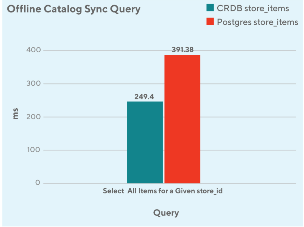
The first example here is as depicted in figure 2: select query performance based on store_id dropped by ~38%. The reason for that is that in CockroachDB, store_id is the first column in the composite primary key; however, it’s just an ordinary secondary index in the PostgreSQL table.

Fig 2: Bulk(10k+ rows) query performance with legacy DB vs CockroachDB.

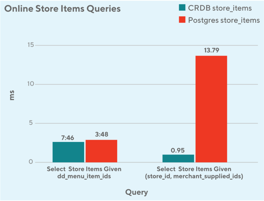
For the rest of online queries as depicted in figure 3, there are two major patterns:

  1. Query against dd_menu_item_ids
    1. It’s designed to be a secondary index for both data stores, the performance is on par
  2. Query against store_id + merchant_supplied_id
    1. It’s the composite key in the CockroachDB table however it’s just a composite secondary index in the PostgreSQL table, the query performance is significantly improved (10x faster) in the CockroachDB compared to the PostgreSQL
Fig 3: Real-time query performance with legacy DB vs CockroachDB.

Conclusion

A scalable backend needs to be backed by a scalable datastore. Any technology has its own pros and cons, and there is no one-size-fits-all solution. What this article presented here is one of the ways to deal with OLTP datastore scalability problem, in the meanwhile we also shared the tech debt in the legacy design, new features adoption in the CockroachDB and how to plan a seamless bug-free migration. Here is the summary:

  1. DoorDash has a recommended size limit 500 GB for a single PostgreSQL table
  2. CockroachDB’s shared-nothing architecture makes it a perfect fit for high resilience, scalability, and support for distributed data and transactions.
  3. Eliminate the tech debt like foreign key, redundant secondary indices, SQL join statements, etc, in the new design
  4. First dual write, then shadow read, and eventually feature-flag-based cutover for a seamless bug-free migration

Those who find themselves in a similar situation of encountering OLTP database scalability bottleneck can take the following steps:

  1. Make your SQL query as simple as possible, move data join from SQL level to the service code, or build a materialized view to store the precomputed join
  2. Use the built-in unique key made up of composite columns in the data itself. This allowed us to forgo the artificial auto-increment key and random generated UUID as unique IDs and save on secondary indices
  3. Use multi-row statements for DML queries to replace multiple single-row statements
  4. Create a facade layer to unify the data access interfaces and isolate the application from the storage engine and facilitate the migration
  5. Understand that CockroachDB is naturally a better choice for applications requiring high resilience, scalability, and support for distributed data and transactions.

This migration allowed us to resolve a lot of legacy tech debt and performance concerns. We are now also in a stage where we can handle 10X load as we continue to scale our new verticals business. 

Contributors:

 Yin Zhang Nikhil Pujari Kevin Chen ThulasiRam Peddineni

App startup time is a critical metric for users, as it’s their first interaction with the app, and even minor improvements can have significant benefits for the user experience. First impressions are a big driver in consumer conversion, and startup times often indicate the app’s overall quality. Furthermore, other companies found that an increase in latency equals a decrease in sales.

At DoorDash, we take app startup speed extremely seriously. We are obsessed with optimizing our customers’ experience and making continuous improvements.

In this article, we will explore three separate optimizations that reduced the time it took to launch our iOS consumer app by 60%. We identified these opportunities using proprietary performance tools, but Xcode instruments or DTrace could also be suitable alternatives.

Changing String(describing:) to ObjectIdentifier()

In early 2022, our app startup optimization journey began with visualizing top bottlenecks using Emerge Tools’ Performance Analysis tool, as seen in Figure 1.

Figure 1: Stack trace showing the three performance optimization opportunities

This performance tool helped showcase unoptimized branches from both a birdseye and a detailed point-of-view. One of the biggest immediate standouts was the time we spent on Swift protocol conformance checks (checking if a type conforms to a protocol), but why?

Architectural principles like the single responsibility principle, separation of concerns, and others, are key to how we write code at DoorDash. Services and dependencies are often injected and described by their type. The problem is that we used String(describing:) to identify services, which came with a runtime performance penalty of checking if the type conforms to various other protocols. The stack trace in Figure 2 is taken directly from our app launch to showcase this.

Figure 2: Stack trace of what happens behind the scenes of the String(describing:) API

The first question we asked ourselves was: “Do we really need a string to identify a type?”Eliminating the string requirement and switching to identifying types using ObjectIdentifier instead, which is a mere pointer to the type, yielded 11% faster app startup times. We also applied this technique to other areas where a pointer sufficed instead of a raw string, which yielded an additional 11% improvement.

If it’s possible to use a raw pointer to the type instead of using String(describing:) We recommend making the same change to save on the latency penalty.

Stop converting unnecessary objects to AnyHashable

At DoorDash, we encapsulate user actions, network requests, data mutations, and other computational workloads into (what we call) commands. For example, when we load a store menu, we submit that as a request to the command execution engine. The engine will then store the command in a processing array and perform the inbound commands sequentially. Structuring our operations this way is a key part of our new architecture, where we purposely isolate direct mutations and observe the results of expected actions instead.

This optimization began with rethinking how we identify commands and generate their hash value. Our processing array, and other dependencies, rely on a unique hash value to identify and separate the respective commands. Historically, we circumvented the need of having to think about hashing by using AnyHashable. However, as noted in the Swift standard, doing so was dangerous because relying on hash values given by AnyHashable could change between releases.

We could have chosen to optimize our hashing strategy in several ways, but we started by rethinking our original restrictions and bounds. Originally, the hash value of a command was a combination of its associated members. This decision had been made deliberately since we wanted to maintain a flexible and powerful abstraction of commands. But after an app-wide adoption of the new architecture, we noticed that the design choice was premature and overall left unused. Changing this requirement to identify commands by their type led to a 29% faster app launch, 55% faster command execution, and 20% faster registration of commands.

Auditing 3rd party framework initializers

At DoorDash, we strive to be free of third-party dependencies wherever possible. Still, there are times when a consumer’s experience could greatly benefit from a third-party integration. Regardless, we conduct several rigorous audits of how third-party dependencies impact our service and the quality we uphold.

A recent audit found that a certain third-party framework caused our iOS application to launch roughly 200ms slower. This framework alone occupied roughly 40%(!) of our app launch time, as seen in Figure 3.

Figure 3: A flame chart showing roughly 200ms of our app startup time was due to a third-party framework iterating over our NSBundle.

To make matters trickier, the framework in question was a key part of ensuring a positive consumer experience. So what can we do? How do we balance one aspect of the customer experience with fast app launch times?

Typically, a good approach is to start by moving any computationally expensive startup functions to a later part of the launch process and reevaluate from there. In our case, we only called or referenced classes in the framework much later in the process, but the framework was still blocking our launch time; why?

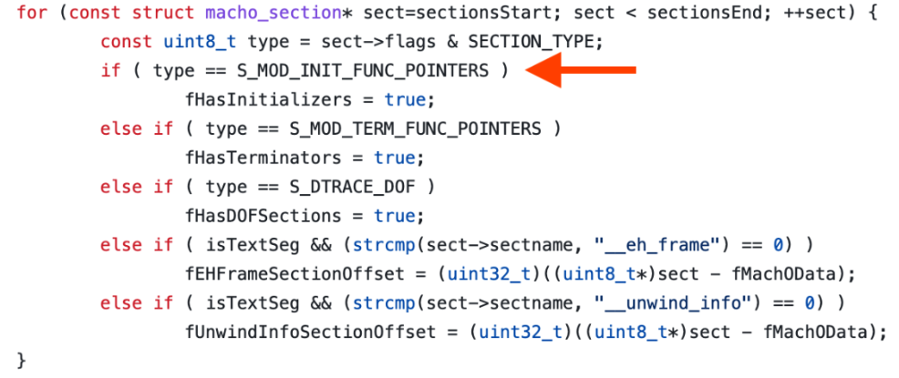
When an application starts up and loads into memory, the dynamic linker (dyld) is responsible for getting it ready. One of the steps of dyld is scanning through dynamically linked frameworks and calling any module initialization functions that it may have. dyld does this by looking for section types marked with 0x9 (S_MOD_INIT_FUNC_POINTERS), typically located in the “__DATA” segment.

Once found, dyld sets a Boolean variable to true and calls the initializers in another phase shortly thereafter.

The third-party framework in question had a total of nine module initializers that all, because of dyld, were granted to run before our application ran main(). Those nine initializers attributed to the total cost that delayed our app launch. So how do we fix it?

There are several ways we could have gone about fixing the delay. A popular option is to use dlopen and write a wrapper interface for functions that have yet to be resolved. This method meant losing compiler safety, though, since the compiler could no longer reassure that a certain function would exist in the framework at compile time. This option has other cons, but compile safety meant the most to us.

We also contacted the third-party developers and asked them to convert the module initializer to a simple function we could instead call at our leisure. They, unfortunately, have yet to reply to us.

Instead, we went for a slightly different approach than publicly known methods. The idea was to trick dyld into thinking it is looking at a regular section and therefore skip calling the module initializers. Then, later at runtime, we would grab the base address of the framework with dladdr, and call the initializers at a known static offset. We would enforce this offset by validating the hash of the framework at compile time, verifying sections at runtime, and checking that the section flag had indeed been replaced. With these safety guards and an overall plan in mind, we successfully rolled out this optimization and yielded an additional 36% faster app startup.

Conclusion

Accurately identifying performance bottlenecks and opportunities is often the most challenging part of any optimization. Notoriously, a common mistake is to measure A, optimize B, and conclude C. That is where good performance tools help highlight bottlenecks and surface them. Xcode instruments, a part of Xcode, come with several templates to help pinpoint various potential issues in a macOS/iOS application. But for additional granularity and ease of use, Emerge Tools provides a simplified view of app performance with their performance tools.

As DoorDash’s business has grown with increasing order volumes and through emerging businesses including grocery delivery, our customer support experience also needed to scale up efficiently. The legacy support application that DoorDash had built to issue credits and refunds was created only to address the original food delivery service. It couldn’t handle the needs of our new verticals. 

We needed a more scalable and automated means of distributing credits and refunds when customer experiences failed to meet our quality guarantees. These new performance requirements could not realistically be added to our legacy credits and refunds service, which operated on our legacy backend framework, Python. Instead, we pursued a complete redesign to upgrade our system, building a no-code platform and migrating the service to Kotlin, our new backend framework. 

In this article, we will walk through how we rewrote the service to solve the challenges inherent in issuing credits and refunds for new verticals. We also discuss how we migrated the system to Kotlin. 

Redesigning the customer support application

Our legacy customer support application utilized a configurator, which is what we call our web-based tool. It allows customer service agents to associate a customer issue with a corresponding resolution strategy. The criteria for selecting resolution strategies was defined in the code. We expected to provide fast, accurate resolutions at relatively low cost with this new customer support platform. We narrowed down the next step for the upgrade to two possible approaches. 

Our first approach would involve continuing to leverage the legacy architecture. Because our engineers developed the legacy application and have a thorough knowledge of it, composing new resolution strategies for the legacy system would be straightforward, streamlining the development work. The tradeoff inherent to this approach, however, is that we would have to rely heavily on the engineers to make continuous code changes to support the customer support team as they adjusted resolution strategies and ran optimization experiments.

Alternatively, we could move the code-defined resolution strategies and experimentation capabilities outside the codebase to make them configurable by non-engineers. A configuration-driven, no-code solution would reduce the reliance on engineers and enable our operators to move faster because they could translate resolution strategies into configurations in a “what you see is what you get” manner. To ensure that this solution would scale with our future business needs, we decided to use a decision tree configuration. This would break down ambiguities because each path in a decision tree can represent a unique resolution strategy. When a new strategy is introduced with the decision tree representation, the configuration can easily extend by adding a new branch to the tree. The downside of this approach is that it requires more up-front investment in resources when compared to just extending the code. We would also need to train operators on how to define strategies and experiments using the self-serve configurator.

Ultimately, we decided that the second approach’s benefits outweigh the drawbacks. Consequently, we elected to redesign the basic customer support application into a configurable no-code platform that can support fast changes and experimentation.       

Migrating the system from Python to Kotlin  

The “componentization” of a credit and refund strategy could be implemented in the legacy Python codebase at the same time we worked to spin up a new Kotlin service. In other words, we could continue to improve the existing application to meet current business needs — a relatively low-cost action — and simultaneously tackle system migration as a separate effort. A fast-growing business requires the fast delivery of technical solutions. Of course, the tradeoff is that failing to address the underlying technical issue means we would continue to build code that adds to our technology debt, not to mention that we eventually would need to deprecate the code. But tackling a large migration effort in a fast-growing environment creates a risk of significant business disruption.

An alternative option would be to stop building new code in our existing Python application to focus exclusively on spinning up our new Kotlin service. As new business requests arose, we could implement those requests in the Kotlin service. This approach would offer the advantage of not building tech debt while steadily migrating code without significant disruption to the business. A key drawback: We would have a hybrid state with both the legacy system and the new system involved. Both systems would have to be maintained and monitored for a longer period of time.

However, one additional factor tipped the balance in favor of Kotlin. DoorDash Engineering’s decision to use Kotlin as its microservices programming language meant that our new service would be operating fully inside DoorDash’s tech ecosystem and infrastructure. 

We chose that second approach and created a new customer support platform in Kotlin while gradually migrating the legacy application over. We believe this path provides the best chance for initiating and completing the systems migration without significantly disrupting our business.

Making the credit and refund strategies configurable  

After we created a new Kotlin service, we defined gRPC endpoints to create and read a credit and refund strategy. Our biggest redesign effort revolved around implementing a credit and refund configurator to allow operators to create credit and refund strategy decision trees (see Figure 1). The configurator required building a visual editor to arrange credit and refund decision trees using a drag-and-drop mechanism and creating APIs to store and fetch configuration data for the trees. In addition to the visual editor, we needed a framework to parse the configuration data and execute the actions that the tree specified. Client services needed an API to invoke this execution framework. But building these capabilities from scratch would be time and cost prohibitive. 

Figure 1: The credit and refund configurator allows operators to configure credit and refund strategies based on a decision tree

Fortunately, we already had a homegrown decision tree-based configuration platform to configure business and technical flows without code. We leveraged this existing workflow platform to store and fetch configuration data for credit and refund strategies. To help operators define those strategies, we also added special types of nodes that could only be understood by the credit and refund platform. For example, the is_vertical_id_in_list node in Figure 1 checks the business vertical. It tells the next node if the order is, for example, a restaurant order, a grocery order, an alcohol order, or a pharmacy order. Based on the output of the is_vertical_id_in_list node, there would be different credit and refund strategies.

We had an experimentation platform at DoorDash, but experiments needed to be hard-coded by engineers. To save engineering time, we enhanced the workflow platform to configure an experiment without code. We added a new type of node, select_control_or_x_treatment (x is the number of treatment groups; see Figure 1), that allows operators to name an experiment. If a select_control_or_x_treatment node is configured as part of a decision tree, the workflow platform will leverage the APIs provided by the experimentation platform to execute the experiment and take the treatment or control path based on the results.

Exploring the technical architecture

At this stage, we were ready to put everything together.

To orchestrate credits and refunds, the Python application routed the traffic to the Kotlin application to determine strategies. The control flow then returned back to the Python application. The architecture behind the customer support platform, as shown in Figure 2, highlights how the Python and Kotlin systems work together to issue credits and refunds. This architecture transformed the way we tested and experimented with customer support resolution strategies.

Figure 2: The architecture behind the customer support platform highlights how the Python and Kotlin systems work together to issue credits and refunds
Figure 2: The architecture behind the customer support platform highlights how the Python and Kotlin systems work together to issue credits and refunds   

Conclusion

After the redesigned system was rolled out, we saw significant improvement in how quickly our operators could respond to customer problems and define, test, experiment, and roll out credit and refund resolution strategies. As the behavior of the system changed, new challenges cropped up, including a need for transparency about the system’s configuration changes made. We also needed more system guardrails because we required stricter validation of the configuration data before it rolled into production. As our configuration-based decision-making system evolves, we are discovering new requirements, including a need for automated testing of resolution strategies to prevent production environment regressions created by inaccurate strategies. 

Migrating systems from one technical stack to another is a complex endeavor. There is a natural temptation to redesign the system as part of the migration to eliminate technology debt and introduce best practices. When we did both at once, we kept an eye on maintaining functional feature parity between the two systems. After the technical migration was completed, we were able to verify that there were no regressions introduced. Subsequently, we cut traffic over to the new system, allowing newer functional requirements to be applied only to the new system.

Acknowledgments

Thanks to Abin Varghese, Han Huang, Kumaril Dave, and Borui Zhang for their contributions to this effort. 

One of the great features of developing in SwiftUI is Xcode Previews which enable rapid UI iteration by rendering code changes in near real-time alongside the SwiftUI code. At DoorDash we make heavy use of Xcode Previews along with the SnapshotTesting library from Point-Free to ensure that screens look how we expect while developing them and ensure they don’t change in unexpected ways over time. SnapshotTesting can be used to capture a rendered image of a View and create an XCTest failure if the new image doesn’t match the reference image on disk. Xcode Previews in combination with SnapshotTesting can be used to provide quick iterations while still ensuring views continue to look the way they’re intended without fear of unexpected changes. 

The challenge of using Xcode Previews and SnapshotTesting together is that it can result in a lot of boilerplate and code duplication between previews and tests. To solve this problem DoorDash engineering developed PreviewSnapshots, an open-source preview snapshot tool that can be used to easily share configurations between Xcode previews and snapshot tests. In this article, we will delve into this topic by first providing some background into how Xcode previews and SnapshotTesting work and then explaining how to use the new open-source tool with illustrative examples of how to remove code duplication by sharing view configurations between previews and snapshots.

How Xcode Previews work

Xcode Previews allow developers to return one or more versions of a View from a PreviewProvider and Xcode will render a live version of the View alongside the implementation code.

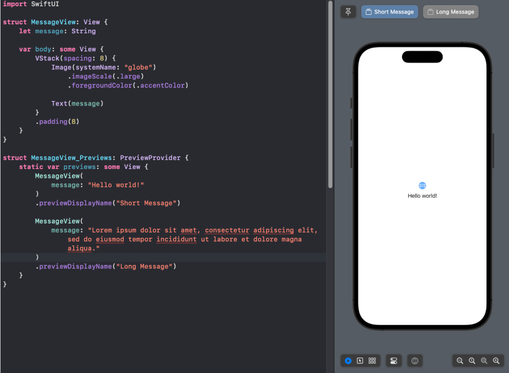
As of Xcode 14 views with multiple previews are presented as selectable tabs along the top of the preview canvas as pictured in Figure 1.

Figure 1: Xcode editor showing SwiftUI View code for displaying a simple message alongside Xcode Preview canvas rendering two versions of that view. One with a short message and one with a long message.

How SnapshotTesting works

The SnapshotTesting library allows developers to write test assertions about the appearance of their views. By asserting that a view matches the reference images on disk, developers can be sure that views don’t change in unexpected ways over time.

The example code in Figure 2 will compare both the short and long versions of MessageView with the reference images stored to disk as testSnapshots.1 and testSnapshots.2 respectively. The snapshots were originally recorded by SnapshotTesting and automatically named after the test function along with the assertion’s position within the function.

Figure 2: Xcode editor showing SwiftUI View code using PreviewSnapshots for generating Xcode Previews for four different input states alongside Xcode Preview canvas rendering the view using each of those states

The problem with using Xcode Previews and SnapshotTesting together

There’s a lot in common between the code used for Xcode Previews and for creating snapshot tests. This similarity can result in code duplication and extra effort for developers when trying to embrace both technologies. Ideally, developers could write code for previewing a view in a variety of configurations and then reuse that code for snapshot testing the view in those same configurations.

Introducing PreviewSnapshots

Solving this code duplication challenge is where PreviewSnapshots can help. PreviewSnapshots allow developers to create a single set of view states for Xcode Previews and create snapshot test cases for each of the states with a single test assertion. Below we will walk through how this works with a simple example. 

Using PreviewSnapshots for a simple view

Let’s say we have a view that takes in a list of names and displays them in some interesting way.

Traditionally we’d want to create a preview for a few interesting states of the view. Perhaps empty, a single name, a short list of names, and a long list of names.

struct NameList_Previews: PreviewProvider {
  static var previews: some View {
    NameList(names: [])
      .previewDisplayName("Empty")
      .previewLayout(.sizeThatFits)

    NameList(names: [“Alice”])
      .previewDisplayName("Single Name")
      .previewLayout(.sizeThatFits)

    NameList(names: [“Alice”, “Bob”, “Charlie”])
      .previewDisplayName("Short List")
      .previewLayout(.sizeThatFits)

    NameList(names: [
      “Alice”,
      “Bob”,
      “Charlie”,
      “David”,
      “Erin”,
      //...
    ])
    .previewDisplayName("Long List")
    .previewLayout(.sizeThatFits)
  }
}

Then we’d write some very similar code for snapshot testing.

final class NameList_SnapshotTests: XCTestCase {
  func test_snapshotEmpty() {
    let view = NameList(names: [])
    assertSnapshot(matching: view, as: .image)
  }

  func test_snapshotSingleName() {
    let view = NameList(names: [“Alice”])
    assertSnapshot(matching: view, as: .image)
  }

  func test_snapshotShortList() {
    let view = NameList(names: [“Alice”, “Bob”, “Charlie”])
    assertSnapshot(matching: view, as: .image)
  }

  func test_snapshotLongList() {
    let view = NameList(names: [
      “Alice”,
      “Bob”,
      “Charlie”,
      “David”,
      “Erin”,
      //...
    ])
    assertSnapshot(matching: view, as: .image)
  }
}

The long list of names could potentially be shared between previews and snapshot testing using a static property, but there’s no avoiding manually writing an individual snapshot test for each state being previewed.

PreviewSnapshots allows developers to define a single collection of interesting configurations, and then trivially reuse them between previews and snapshot tests.

Here is what an Xcode preview looks like using PreviewSnapshots: 

struct NameList_Previews: PreviewProvider {
  static var previews: some View {
    snapshots.previews.previewLayout(.sizeThatFits)
  }

  static var snapshots: PreviewSnapshots<[String]> {
    PreviewSnapshots(
      configurations: [
        .init(name: "Empty", state: []),
        .init(name: "Single Name", state: [“Alice”]),
        .init(name: "Short List", state: [“Alice”, “Bob”, “Charlie”]),
        .init(name: "Long List", state: [
          “Alice”,
          “Bob”,
          “Charlie”,
          “David”,
          “Erin”,
          //...
        ]),
      ],
      configure: { names in NameList(names: names) }
    )
  }
}

To create a collection of PreviewSnapshots we construct an instance of PreviewSnapshots with an array of configurations along with a configure function to set up the view for a given configuration. A configuration consists of a name, along with an instance of State that will be used to configure the view. In this case, the state type is [String] for the array of names.

To generate the previews we return snapshots.previews from the standard previews static property as illustrated in Figure 3. snapshots.previews will generate a properly named preview for every configuration of the PreviewSnapshots.

Figure 3: Xcode editor showing SwiftUI View code using PreviewSnapshots for generating Xcode Previews for four different input states alongside Xcode Preview canvas rendering the view using each of those states

For a small view that’s easy to construct, PreviewSnapshots provides some additional structure but doesn’t do much to reduce the lines of code within previews. The major benefit for small views comes when it’s time to write snapshot tests for the view.

final class NameList_SnapshotTests: XCTestCase {
  func test_snapshot() {
    NameList_Previews.snapshots.assertSnapshots()
  }
}

That single assertion will snapshot test every configuration in the PreviewSnapshots. Figure 4 shows the example code alongside the reference images in Xcode. Additionally, if any new configurations are added in the previews they will automatically be snapshot tested with no change to the test code.

Figure 4: Xcode unit test using PreviewSnapshots to test four different input states defined above with a single call to `assertSnapshots`
Figure 4: Xcode unit test using PreviewSnapshots to test four different input states defined above with a single call to assertSnapshots

For more complex views with lots of arguments, there’s even more benefit.

Using PreviewSnapshots for a more complex view

In our second example we take a look at a FormView which takes several Bindings , an optional error message, and an action closure as arguments to its initializer. This will demonstrate the increased benefits of PreviewSnapshots as the complexity of constructing the view increases.

struct FormView: View {
  init(
    firstName: Binding<String>,
    lastName: Binding<String>,
    email: Binding<String>,
    errorMessage: String?,
    submitTapped: @escaping () -> Void
  ) { ... }

  // ...
}

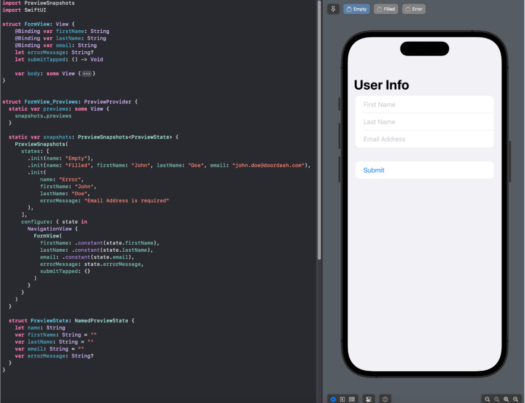
Since PreviewSnapshots is generic over the input state we can bundle up the various input parameters into a small helper structure to pass into the configure block and only have to do the work of constructing a FormView once. As an added convenience PreviewSnapshots provides a NamedPreviewState protocol to simplify constructing input configurations by grouping the preview name along with the preview state.

struct FormView_Previews: PreviewProvider {
  static var previews: some View {
    snapshots.previews
  }

  static var snapshots: PreviewSnapshots<PreviewState> {
    PreviewSnapshots(
      states: [
        .init(name: "Empty"),
        .init(
          name: "Filled",
          firstName: "John", lastName: "Doe", email: "[email protected]"
        ),
        .init(
          name: "Error",
          firstName: "John", lastName: "Doe", errorMessage: "Email Address is required"
        ),
      ],
      configure: { state in
        NavigationView {
          FormView(
            firstName: .constant(state.firstName),
            lastName: .constant(state.lastName),
            email: .constant(state.email),
            errorMessage: state.errorMessage,
            submitTapped: {}
          )
        }
      }
    )
  }
  
  struct PreviewState: NamedPreviewState {
    let name: String
    var firstName: String = ""
    var lastName: String = ""
    var email: String = ""
    var errorMessage: String?
  }
}

In the example code we created a PreviewState structure that conforms to NamedPreviewState to hold the name of the preview along with the first name, last name, email address, and optional error message to construct the view. Then in the configure block we create a single instance of FormView based on the configuration state passed in. By returning snapshots.preview from PreviewProvider.previews, PreviewSnapshots will loop over the input states and construct a properly named Xcode preview for each state as seen in Figure 5. 

Figure 5: Xcode editor showing SwiftUI View code using PreviewSnapshots for generating Xcode Previews for three different input states alongside Xcode Preview canvas rendering the view using each of those states

Once we’ve defined a set of PreviewSnapshots for previews we can again create a set of snapshot tests with a single unit test assertion.

final class FormView_SnapshotTests: XCTestCase {
  func test_snapshot() {
    FormView_Previews.snapshots.assertSnapshots()
  }
}

As with the simpler example above this test case will compare each of the preview states defined in FormView_Previews.snapshots against the reference image recorded to disk and generate a test failure if the images don’t match the expectation.

Conclusion

This article has discussed some of the benefits of using Xcode Previews and SnapshotTesting when developing with SwiftUI. It also demonstrated some of the pain points and code duplication that can result from using those two technologies together and how PreviewSnapshots allows developers to save time by reusing the effort they put into writing Xcode previews for snapshot testing. 

Instructions for incorporating PreviewSnapshots into your project, as well as an example app making use of PreviewSnapshots, are available on GitHub.

One challenge in running our platform is being able to accurately track Merchants’ operational status and ability to receive and fulfill orders. For example, when a Merchant’s location is physically closed but marked as open on our platform, we might create a bad experience for all of our users; a Dasher cannot complete their accepted delivery, the Consumer cannot receive their ordered food, and the Merchant could see lower future revenues. Similarly, when a Merchant who is open but marked as closed on our platform results in similarly negative outcomes; Consumers can not make an order, the Merchant loses potential revenue, and Dashers lose potential delivery opportunities as well. 

This post will highlight how we used machine learning to predict the operational status of a store and deliver the best possible experience for Merchants, Dashers, and Customers. 

The challenge of having accurate store operational hours 

On the DoorDash marketplace stores operate independently, which means that we do not always get the most up-to-date information on merchant’s business hours and operational status. Not having accurate operational hours is an acute problem when merchants are dealing with staffing and supply-chain shortages. Therefore, in a small percentage of deliveries, the Dasher might find that the store is actually closed. With tens of millions of deliveries being fulfilled each week, quickly and efficiently confirming such merchant closures and reacting to them is key for these reasons:

  • To allow consumers to quickly be informed of the issue and get refunded. 
  • To make sure that no further orders can be placed at a closed store.

However, leveraging our support team to act on these Dasher-reported closures is both costly and inefficient, given the thousands of closed store cases that are reported each day. To help Dashers quickly resolve closed merchant issues with maximum efficiency, we built a “Dasher reports store closed” feature [DRSC for short] directly in the Dasher app. In the rest of the article, we will walk through how this feature works and how we augmented it with ML to improve its performance and automation. 

How the DRSC works 

When Dashers find themselves unable to pick up an order at a store location that appears closed, they are prompted to take a picture of the store to kick off the reporting process. When a valid picture is uploaded, the Dasher is compensated for the partial time and effort they spent getting to the store, and are unassigned from the delivery so that they can continue their dash and be assigned other deliveries. 

Figure 1. The Dasher app powers the automated DRSC report.

When a DRSC report is received, a set of actions can be taken on the order: we could either cancel the delivery and reimburse the customer, or alternatively when we have reason to doubt the report’s accuracy we could reassign the order to a new Dasher to re-attempt the pickup.

In parallel, we need to contact the merchant to confirm that the store is indeed closed, so we can pause it on the platform. If the merchant confirms the closure or is unresponsive, we will pause the store for a set period of time. Pausing the merchant prevents consumers and Dashers from unnecessarily experiencing another similar issue when we already have some signal information that the store is closed. If the Merchant confirms the store is open, then the report is rejected, we find a different Dasher to fulfill this order, and the merchant can continue receiving other orders. 

The existence of inaccurate reports, though infrequent, is a major challenge for DRSC that we set out to minimize using ML.

Why we went the ML route

Without carefully examining each DRSC report, we might unnecessarily cancel orders or pause merchants. We needed an ML-powered solution to automate this review process at scale. Since some DRSC reports are inaccurate, either because the image does not show a closed store or the merchant confirms they are in fact open, having a trusted means of reviewing the DRSC validities meant we would be better equipped to reassign another Dasher and complete the order, when the validity of the DRSC report is in question. 

A validation step that can categorize reports would need to be accurate and fast, and scale up to thousands of daily reports. Humans could do it, but it would be expensive, time-consuming, and unscalable. A heuristic set of rules could handle the required speed and scale but would be only moderately accurate, with errors in passing inaccurate reports being costly to merchants and painful for customers. Given the inherent uncertainty of the problem, a conditional probability model – a mathematical formula for assigning probabilities to outcomes given varying information – seems especially fit for the job. This is because conditional probability models can pool available information about a store and a Dasher to output inferences about the store status that help us make optimal decisions.

Stay Informed with Weekly Updates

Subscribe to our Engineering blog to get regular updates on all the coolest projects our team is working on

How the ML model replaced the heuristic

We started with the idea of wanting to calculate the probability that a given store is closed when a DRSC report is filed,

Probability(Store is Closed | DRSC report).

While a more general model for inferring store status could be built, we constrained ourselves to only handling the DRSC use case. 

Our first challenge was that the dependent variable (the status of a store) is unknown and would be prohibitively expensive to measure (i.e we do not actually know if a store is closed or not). To construct the store status variable, we looked at past DRSC reports and checked if such stores were fulfilling orders or responding to our messages about the store status in the hour following a DRSC report. For example, when a Dasher is able to complete a pick up within 15 minutes of a historical DRSC report, we would infer that the store was probably still open, despite the report.

A DRSC report provides basic features like the store Id, Dasher Id, timestamp of the report, as well as an image of the storefront taken by the Dasher. Store and Dasher Ids are useful for connecting a DRSC report to a history of deliveries at the store and a history of deliveries across stores by the Dasher. Historical data allows us to build features like the number of recent reports for a given store, the last time a pickup occurred, and the number of invalid store-closed reports for a given Dasher over multiple months.

Additionally, an image of the storefront might contain valuable information about its status by capturing a sign on the door indicating that it’s closed or showing that lights are off. By converting images into a summary signal such as the probability that a ‘store is closed’ or a ‘store is open’ we can process and use hundreds of thousands of images quickly. We accomplished this by training an image classifier using our internal image processing platform. The image classifier compresses the image information into a single number which we then use as one of our model features.

Figure 2. The DRSC ML model inputs and output action-set

Finally, a single LightGBM model can combine historical and image information to compute a probability that a store is closed. The probability sets us up to make decisions. Today, we use thresholds to partition the 0-1 probability set into intervals that map onto our actions:

  • low probability of a store being closed leads to unassign the order and find a new Dasher 
  • intermediate probabilities would lead us to cancel the order
  • high probabilities would lead us to both cancel the order and pause the store. 

Following the deployment of this ML model and an AB experiment, we confirmed that the improved decision-making now saves thousands of deliveries from being canceled every week. Avoiding cancellations produces a better consumer experience, increased revenue for our partner merchants, more earning opportunities for Dashers, and a more robust business for DoorDash. This initiative is an example of how automated statistical decision-making can be used to build intelligent logistics infrastructure and provide value for all participants in the marketplace.

Next step: building a dynamic loss function

The next major iteration is making the decision thresholds dynamic. By incorporating time of day, future store volume, and potential future cancellations, we could fine-tune our decision-making when a DRSC report is received. We could then construct a loss function that outputs for each action and store-status a cost we will pay. A loss function and a probability model can be used to compute expected loss and find an action that minimizes it. Effectively, we will have implicit dynamic thresholds that adjust to time and conditions for each store. Being sensitive to cost for each Dasher and Merchant will make our decisions even more effective. 

Conclusion

Many companies have built their operations on heuristics or simple rules. Rules are the quickest route to prove that a problem is solvable by moving from nothing to functional performance. However, there can be a large opportunity cost in not considering upgrading the heuristic solution into an optimized ML solution that will boost the performance to a near-maximum level. Using simple and low-effort ML tools like LightGBM is a great way to start your journey from simple rules to intelligent infrastructure and maximize efficiency. 

In order to inspire DoorDash consumers to order from the platform there are few tools more powerful than a compelling image, which raises the questions: what is the best image to show each customer, and how can we build a model to determine that programmatically using each merchant’s available images?

Figure 1: Discovery surfaces with merchant images

Out of all the different information presented on the home page (see Figure 1), studies with consumers have repeatedly shown that images play the most important role in providing consumers with “evidence” that helps them choose a merchant and which items to order. When consumers evaluate an unfamiliar restaurant, they first think “Does it look good?” Essentially, people eat with their eyes and images can tell them a lot about the food’s cuisine, type of restaurant, quality of food, nutritional information, price range, and more. Once they determine that an item looks good, consumers will continue the ordering journey and access other factors such as type of food, wait time, affordability, etc.

Given the importance of merchant images shown in the studies, we decided to start the project to optimize the merchant image shown to consumers. We want to build a model that will choose the product images that will best entice and inspire consumers. We also wanted to build an exploration model to keep expanding our understanding of which images interest customers.

How we grew our image selection models

How we grew our image selection from an MVP to its current progress exemplifies our team’s practice of starting small and then using data and testing to grow progressively. At the beginning, the image selection logic was simple. We showed the header image for a store in a carousel which is manually selected by operators at the store or business level and showed the image of the best-selling item of the store in store feed and search feed. With the setting, consumers only see a single image across various discovery surfaces. The selected image remained static as it represented the store’s best selling item which had minimal variance over time. In addition, there is a pitfall of the image selection logic, which is that the most bought item may not be an entree or terribly representative of a store. It’s not uncommon for a popular side like fries or a soda to be featured instead of an entree that would better represent the merchant’s offerings. 

How we progressed beyond the MVP

The MVP we built was a positive first step, but after collecting data about the product’s shortcomings, our team went about making improvements for the next iteration. The personalization team first built an image filtration to filter out common items that might not be representative of the merchant. This was done by putting in business rules for restaurants that featured images, should not be drinks or sides (unless that was the merchant’s primary selling point), and saw improvement on key metrics such as conversion in the A/B test.

As the next step, we tested rotating discovery images from a pool of four images (one header image and three most-selling dishes), to showcase a wider selection of best selling items from the store menu. Figure 2 shows an example of an image pool of a merchant. The team hypothesized that showing fresher images will help consumers reconsider a merchant they had previously passed over. The goals were to: 

  • determine if image rotation improved consumer engagement (clicks);
  • determine if image rotation encouraged consumers to try new merchants; 
  • determine whether the combination of the two above improved conversion rate; and
  •  collect training data for machine learning algorithms. 
Figure 2: An example of the pool for image selection which consists of the header image and featured item images. The header image is the image shown on the top of the store page and featured item images are images from the feature items.

The test drove improvements in homepage clicks and new restaurant trials but had a negative impact on homepage conversions. What this means is that fresher images attracted more consumer interest and drove click-throughs to merchant pages. However, fresh images didn’t guarantee conversion. While rotated images piqued consumers’ interest, consumers might be confused that previously rejected merchants showed up differently on their feeds, and opted to reject the same merchants again. The additional friction (rejecting the same merchant again) took away the time consumers could have used on exploring other merchants they are more likely to order from. Therefore the overall homepage conversion dropped. The lesson we learned from here is that there is a difference between what drives click and what drives conversion.

Selecting the best image for each merchant

To address the shortcoming of image rotation, we need to select an image which has high quality and can really drive conversion. Recall that the image pool consists of images from featured (top selling) items. Another challenge we had to deal with was that just because an item was a top seller did not mean it had a high-quality or compelling image. These low-quality images could potentially be bad representatives of the merchant’s selection and items and showing them on the discovery surfaces may actually hurt the conversion rate.

To solve the problem, we used a data driven approach to answer the question: if we need to choose one single image to represent a merchant, what would be the best image? Given that the team’s goal is to improve the conversion rate, it’s straightforward to look at past data to figure out which image drove most conversions. The image rotation experiment mentioned above provided us with the data we needed to start the image optimization process.

Balancing exploitation with exploration

Choosing the image which drove the most conversions in the image rotation experiment might be a good start. However, we cannot just choose the images from a previous one-time analysis. The following are the key problems that a simple approach runs into, and which we solved:

  • New images don’t have a chance to be shown to consumers. The initial conversion rate is 0 for a new image but it may be an image with high quality.
  • Consumers’ taste may change over time. The image which drove most conversion in the past is not guaranteed to drive most conversion in the future. If we always show the image, there is no chance for other images to catch up.
  • Consumers may get tired of seeing the same image again and again. If the consumer doesn’t find the current image attractive, showing the same image may not help conversion.

To introduce exploration, we used a multi-arm bandit algorithm to implement the Image EnE model. The approach is similar to what we did in Homepage Recommendation with Exploitation and Exploration

The composite (final) model score is formulated as:

where:

  • c is the consumer id
  • m is the merchant id
  • i is the image url

where:

The exploitation score is the conversion rate (CVR score) for the image, aggregated over all consumers for each image. The exploration score is based on the number of impressions the consumer had on the image. The more impressions, the lower the score. The Image EnE model introduces uncertainty to the CVR score with a multiplier CENE to balance between exploitation and exploration.

We then select the image with the highest composite model score to display to the consumer. Both the exploitation term and exploration term contribute to the composite score. To explore an illustration of each contribution:

  • For a given consumer, we explore until we find an image that converts. For example, the consumer saw image A on day one as it has the highest score on the day. The consumer had seen image A for several days but didn’t convert. Due to the impression discount, image B, with the second-best conversion rate, has a higher composite score than A on day three and has been surfaced to the consumer since then. 
  • Because we are always exploring, we learn when the global performance of images changes and do not lock into one image. Image A had the highest conversion rate on day one. However, the conversion rate dropped over time because consumers’ taste changed. Another image can have higher conversion rate and thus higher composite score than image A. The exploitation and exploration mechanism ensures fair competition among images and freshness of the images.

As a result, the explore-exploit model finds the most compelling image for a merchant from a pool of six images (five top selling items + header image) for every user session. Instead of exploiting one image, the model regularly surfaces a fresh image to consumers to explore and get feedback. As a consumer engages or does not engage with the merchant, the model learns their preferences and adjusts the image for the merchant. For instance,

  • If a consumer does not convert on image A from a merchant, the model surfaces a different image B to gather feedback.
  • If a consumer converts on image A from a merchant, the model then fixes the image with no future changes for this merchant-consumer pair to ensure recognizability.
  • As the model collects feedback from all consumers, the “exploit” component of the model scales the highest conversion image (say image C) to all consumers.

Stay Informed with Weekly Updates

Subscribe to our Engineering blog to get regular updates on all the coolest projects our team is working on

Choosing the right tradeoff between exploitation and exploration

The multiplier CENE in the above formula controls the tradeoff between exploitation and exploration. To have a good product experience, we have to choose the multiplier appropriately. We can do an A/B test to determine the optimal value of the multiplier. However, A/B experiments take time and we need to ensure enough traffic for each treatment group. Therefore we cannot have too many treatment groups and multipliers to test. We have to narrow down our search space for the multipliers.

Before the A/B test, we analyzed the past data from the Image Rotation experiment. In the past data, we know the CVR score for each image. Therefore, for each merchant, we can simulate the image replacement process–that is, after how many impressions would the composite score be discounted enough such that the previously second-best image becomes the best. Aggregating over all merchants, we have the probability of image change after X views with different multipliers. We wrote code to run the analysis on past data so we can estimate the probability with as many multipliers as we want.

When the uncertainty multiplier is 0, there is no uncertainty and exploration, so the probability of image change is 0 regardless of the number of views. When the uncertainty multiplier is very high such as 0.05, there is more weight on the exploration term, making image change frequently; merchants would change images after 3 views when the multiplier is 0.05. Based on the data, we decided to test two variants in the first A/B test, one with multiplier=0 and the other with multiplier=0.01. We ran the A/B test for several weeks and saw improvement on new restaurant trials while maintaining conversion rate and order frequency.

Figure 3 shows examples where the model improved the image quality:

Figure 3: Before and after applying the Image EnE algorithm

Contextualizing the image with the search query

The above paragraphs describe how we select an image for each merchant without any context such as consumer intent, time of day, and so on. We believe selecting an image that matches the current context is also important. To begin with, we started with the search query. When a consumer searches for a dish, there is a strong intent to order that dish. On average, these queries underperform merchant name searches in conversion. 

We hypothesized that this may be happening due to friction in finding the dishes consumers are craving in that moment: 

  • When consumers search for a specific dish (e.g. burger), images of other dishes are surfaced on the search feed, necessitating a click through to the store to see if the merchant serves that dish.
  • Even after landing on the store page, consumers have to scroll to find the dish.

Therefore, Search and Personalization teams tested:

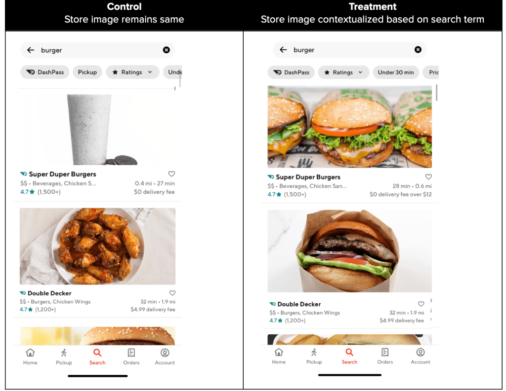
  • Surfacing contextualized images on the search feed that includes the best selling item related to what a consumer has searched with a goal to pique their interest and improve the click-through at the very first glance, especially for an unfamiliar store (Figure 4). 
  • Showing a carousel on top of the store page featuring items related to what the customer has searched for with an objective of reducing the friction of scrolling through the entire menu and improving conversion (Figure 5).

To power this feature we matched against item tags provided by the food catalog. We tested the feature together as: (1) we wanted to test the end state and we posited that both features together would have a higher volume impact (the image optimization would improve search CTR while the carousel would improve conversion), and (2) we had limited traffic to test against (7 search terms) – we would index on funnel metrics to help inform if both parts of the experience were successful.

User Experience

Figure 4: The control (left) and treatment (right) user experience on the search feed
Figure 5: The control (left) and treatment (right) user experience on the store page

The A/B test showed a neutral impact on search conversion, probably because we were limited to the seven search terms (dish types) where the food catalog had high precision and recall. We will continue to improve the precision and recall of the food catalog, expand to more dish types, and iterate the product.

Future work

Our journey on Image Personalization doesn’t end here. There are many aspects where we can improve our system and algorithms. Below we describe some ideas for the next phases in the future.

  • Rule-based, more contextual/consumer feature: similar to what we did for search context, we can start with a rule-based approach to boost images which fit other contexts or filter out images which don’t fit the contexts.
  • ML-based Image Personalization: we will go beyond a rule-based boost or filter and use machine learning to predict a score from the features. We will use historical data to train the model to predict a score based on more features. The score will be used as the exploitation score in the Image EnE framework described in the article, replacing the status quo which is conversion rate among all consumers. 
  • Content Personalization: Once we prove the success of image personalization, we will expand our expertise and experience from Image Personalization to other content on the discovery surfaces.

Conclusion

In the article, we explained the discovery surfaces on DoorDash, why having a good image on these discovery surfaces is important, and the goal of Image Personalization. Then we described how we start Image Personalization with Image Rotation to collect data and early signals. Next, we talked about why we need a balance between exploitation and exploration for images and how we achieve it. We introduced the reinforcement learning algorithm UCB and described how we use UCB in the Image Exploitation and Exploration (EnE) model. We also explained how we selected the multiplier to tradeoff exploitation and exploration and how we conducted A/B tests. We also introduced the concept of selecting images based on the context and described the experiment we did for search context. Finally, we talked about the future work of Image Personalization.

Acknowledgments

Many thanks to Parul Khurana, Josh Zhu, Yu Zhang, Mengjiao Zhang, Jay Zhang, Chen Dong, Di Li, and Sandor Nyako for sharing their insights on the development, and support for the execution of the ideas in this blog post. Our gratitude also goes to Elena Lin and Jessica Zhang for the data-driven insights and for helping us develop the experiment strategy and measurement framework. Special thanks Ezra Berger for the continuous support, review, and editing of this article.

Building software today can require working on the server side and client side, but building isomorphic JavaScript libraries can be a challenge if unaware of some particular issues, which can involve picking the right dependencies and selectively importing them among others.

For context, Isomorphic JavaScript, also known as Universal JavaScript, is JavaScript code that can run in any environment — including Node.js or web browser. The alternative to Isomorphic JavaScript is creating separate, targeted libraries for each environment, for instance one for Node.js and one for the browser. Having a single library across environments offers straightforward benefits — if you can tackle the challenges involved in building one.

Why build isomorphic libraries? 

Like many platform teams, the web platform team at DoorDash builds and maintains several libraries aimed at improving front-end developer productivity. Developers at DoorDash write code in multiple JavaScript environments, including React apps and Node.js web services. Furthermore, DoorDash is migrating several pages from being client-side rendered to server-side rendered so the line between which environment code is run in is increasingly blurry. All of these reasons make a strong case that we should make many of our libraries isomorphic because the same logic needs to work in many different environments.

However, there is also additional complexity involved in supporting multiple environments. This complexity is placed on the library’s creator, not its adopter. For some use cases, this trade-off of complexity vs efficiency may not be worth it.

To illustrate some of these additional complexities, we will walk through the process of building a simple fictitious isomorphic library using code snippets and then highlight five specific challenges. Our goal is to provide context that will be helpful in evaluating whether it makes sense to build an upcoming library isomorphically. We also will show some techniques that can be employed to tackle these challenges.

Isomorphic library example functional requirements

Note: The following is written in Typescript, which compiles to JavaScript, so it may include some typing challenges that are not relevant to those written directly in JavaScript. 

As mentioned in the previous section, this blog post will dive into how to build a fictitious isomorphic library. To pick a good topic for this fake library, let’s first consider what makes isomorphic libraries challenging, namely having to handle environment-specific cases. Some examples of this challenge may be:

  • Relying on any APIs that are native in one environment (for the browser it could be `document.cookies`, `fetch`, etc.) but not native in another
  • Having dependencies that are not isomorphic
  • Functions that behave differently depending on the environment
  • Exposing parameters that are not needed in all environments

Because this blog post focuses on illustrating the challenges of isomorphic JavaScript, our fictitious library has all of these traits. To summarize what we are going to build: a library that exports one function that checks if a coffee order is ready by making a network request and sending a unique id. More specifically, this example has all of the following requirements:

  • Exports a single async function named `isCoffeeOrderReady` which optionally takes `deviceId` as a parameter and returns a Boolean
  • Sends an http POST request with the request body ‘{deviceId: <deviceId>}’ to a hard-coded endpoint
  • Can run in Node.js or browser
  • The browser will read the `deviceId` directly from cookies
  • Uses keep-alive connections

Now that the details of what this fictitious library will do has been scoped out, let’s dive into the five primary challenges that may be encountered in isomorphic library development, and how to tackle them.

Challenge #1: Choosing the right dependencies

For the sake of illustration, assume that this is Node <=16 and that it doesn’t use any experimental flags. Node 18 has native fetch support.

First we must determine how to make a fetch request. The browser can send a fetch request natively, but to support Node.js, either an isomorphic library or a Node.js library will be used. If an isomorphic library is chosen, it will have to fulfill every environment’s requirements for dependencies. In this case, the chosen library may be scrutinized on its impact on bundle size in the browser.

For simplicity’s sake, we’ll use isomorphic-fetch, which uses node-fetch internally in Node.js and the GitHub fetch polyfill in browsers. The following code illustrates how to make the fetch request:

import fetch from 'isomorphic-fetch'
 
// Request: { deviceId: '111111' }
// Response: { isCoffeeOrderReady: true }
export const isCoffeeOrderReady = async (deviceId: string): Promise<boolean> => {
 const response = await fetch('https://<some-endpoint>.com/<some-path>', {
   method: 'POST',
   body: JSON.stringify({ deviceId })
 })
 return (await response.json()).isCoffeeOrderReady
}

Note: For the sake of brevity, many important details such as retry and error handling will be ignored.

Accessing document.cookie

The code at this point ignores many requirements. For instance, in Node.js the parameter `deviceId` will be used as the deviceId that’s sent in the fetch request, but in the browser the `deviceId` should be read directly from a cookie.

To check whether it is in the browser — which means that document.cookie should be defined — see whether the window is defined; `window` always should be defined in the browser and not defined globally in Node. This code snippet looks like:

`typeof window === “undefined”`.

While this is not the only way of detecting whether code is on the server or client, it is a popular way. Many answers in Stack Overflow or in blog posts use this approach.

The full updated code looks like the sample below:

import fetch from 'isomorphic-fetch'
import * as cookie from 'cookie'
 
export const isCoffeeOrderReady = async (deviceId: string): Promise<boolean> => {
 let id = deviceId
 if (typeof window !== 'undefined') {
   const cookies = cookie.parse(document?.cookie)
   id = cookies.deviceId
 }
 const response = await fetch('https://<some-endpoint>.com/<some-path>', {
   method: 'POST',
   body: JSON.stringify({ deviceId: id })
 })
 return (await response.json()).isCoffeeOrderReady
}

While we now are closer to matching the library’s requirements, we have introduced two more challenges to explore…

Challenge #2: Designing a unified API between environments

The previous code change still requires that the `isCoffeeOrderReady` function have a `deviceId` parameter because it is needed in Node.js environments, but the value is ignored in the browser. Instead, the `deviceId` value is read directly from a cookie. The function declaration for both environments should be different — in browsers the function should take no arguments, but in Node it should require one argument — but given that it is isomorphic, it can’t. So the remaining options are:

  • The API can be written as shown, requiring `deviceId.` But this action may be misleading to adopters because that value must be passed in the browser, even though it will be ignored; or 
  • Make `deviceId` optional. This option means that in the browser environment it can be called with no arguments and in the Node environment it can be called with a `deviceId.` However, this also means that the function can be called in Node.js without an argument; Typescript’s static analysis cannot prevent this misuse of the API.

Although the second approach may be the better choice, that fact could weigh against making this library isomorphic, given that the API usage is different between environments.

Stay Informed with Weekly Updates

Subscribe to our Engineering blog to get regular updates on all the coolest projects our team is working on

Challenge #3: Ensuring dependencies only affect intended environments

This `document.cookie` code change also introduced another issue: `cookie` will be installed in Node.js environments despite not being used at all in the Node.js code path. Granted, installing unnecessary dependencies in Node.js is not nearly as detrimental as installing unnecessary dependencies in the browser, given the importance of maintaining a minimal bundle size. However, it is still important to ensure that unnecessary dependencies are not included in a given environment.

One way to fix this issue is to create separate index files for Node.js and browser and use a bundler — for example, webpack — that supports tree shaking. Afterward, make sure that the environment-specific dependencies are only in the necessary code paths. We will show the code needed to do this in the next section.

Using keep-alive connections

Although it may seem straightforward at first to implement keep-alive connections, it is actually challenging. This goes back to our first challenge in choosing the right dependencies. node-fetch does not implement an identical spec as native browser fetch; one place that the specs differ is in keep-alive connections. To use a keep-alive connection in browser fetch, add the flag:

fetch(url, { …, keepalive: true })

In node-fetch, however, create `http` and/or `https` http.Agent instances and pass that as an agent argument to the fetch request as shown here:

const httpAgent = new http.Agent({ keepAlive: true })
const httpsAgent = new https.Agent({ keepAlive: true })
fetch(url, { agent: (url) => {
 if (url.protocol === "http:") {
   return httpAgent
 } else {
   return httpsAgent
 }
}})

Here the isomorphic-fetch utilizes node-fetch internally but does not expose the agent option. This means that in Node.js environments, keep-alive connections cannot be set up correctly with isomorphic-fetch. Consequently, our next step must be to use the node-fetch and native fetch libraries separately.

In order to use node-fetch and native fetch separately, and keep the environment-specific code path separate, entry points can be used. An example of setting this up in webpack with Typescript looks like this:

package.json

{
   "main": "lib/index.js",
   "browser": "lib/browser.js",
   "typings": "lib/index.d.ts",
   ...
}

Also note that even though “main” for Node.js and “browser” point to different index files, only one type declaration file can be used. This makes sense given that the goal of an isomorphic library is to expose the same API regardless of the environment.

As a reference, here is a list of some isomorphic javascript libraries that use this pattern specifically for the purposes of having an isomorphic fetch:

The final steps create the Node.js and browser code paths using everything previously discussed. For the sake of simplicity, we will name the files “index.ts” and “browser.ts” to match the files in the example “package.json”, but note that it is a bad practice to include logic inside of an index file.

index.ts

import fetch from 'node-fetch'
import http from 'http'
import https from 'https'
import { SOME_URL } from './constants'
const httpAgent = new http.Agent({ keepAlive: true })
const httpsAgent = new https.Agent({ keepAlive: true })
 
type CoffeeOrderResponse = { isCoffeeOrderReady: boolean }
 
export const isCoffeeOrderReady = async (deviceId?: string): Promise<boolean> => {
 if (!deviceId) {
   // can throw error, etc. just need to handle undefined deviceId case
   return false
 }
 const response = await fetch(SOME_URL, {
   method: 'POST',
   agent: (url: URL) => {
     if (url.protocol === "http:") {
       return httpAgent
     } else {
       return httpsAgent
     }
   },
   body: JSON.stringify({ deviceId })
 })
 const json = await response.json() as CoffeeOrderResponse
 return json.isCoffeeOrderReady
}

browser.ts

import * as cookie from 'cookie'
import { SOME_URL } from './constants'
export const isCoffeeOrderReady = async (deviceId?: string): Promise<boolean> => {
 let id = deviceId
 // still keep this check in for safety
 if (typeof window !== 'undefined') {
   const cookies = cookie.parse(document?.cookie)
   id = cookies.deviceId
 }
 const response = await fetch(SOME_URL, {
   method: 'POST',
   keepalive: true,
   body: JSON.stringify({ deviceId: id })
 })
 return (await response.json()).isCoffeeOrderReady
}

With the creation of these files, all of the library’s functional requirements are complete. In this particular library, there is little shared code, so isomorphism’s benefits aren’t showcased. But it is easy to imagine how larger projects would share plenty of code between environments. It is also important to be certain that everything exported has the exact same API because only one list of type declaration files will be published.

Challenge #4: Testing every environment

Now that the library is completed, it is time to add testing. Most tests will need to be written twice to make sure that everything functions correctly in each environment. Isomorphism couples logic across all environments, changes in one environment now must be tested in every environment. There can be additional challenges in testing isomorphic libraries in realistic scenarios. For example, Jest only has experimental support for ESM.

Challenge #5: Observability — metrics and logging

The final thing to consider is metrics, logging, and other pieces of observability. Infrastructure for observability looks very different in each environment. In this example, the library in Node.js may be extended to capture all sorts of metrics, including latency of request, error rate, and circuit breakers, as well as log warnings and errors with context to help trace across microservices. But in the browser, the library may be expanded to only capture errors. These differences can be resolved by using some of the same problem-solving patterns presented earlier. Nonetheless, it is worth noting this large space where implementations are likely to diverge.

Final thoughts

Several challenges arose in even this very simple, fictitious isomorphic library, including:

  • Choosing the right dependencies
  • Designing a unified API between environments
  • Ensuring dependencies only affect intended environments
  • Testing every environment
  • Observability — metrics and logging

We also explored whether the benefits of isomorphism are outweighed by some of the compromises and challenges involved. By keeping these challenges in mind as the isomorphic decision is made, it is possible to develop workable solutions.

As DoorDash’s business grows, engineers strive for a better network infrastructure to ensure more third-party services could be integrated into our system while keeping data securely transmitted. Due to security and compliance concerns, some vendors handling such sensitive data cannot expose services to the public Internet and therefore host their own on-premise data centers. To integrate with such vendors, the DoorDash core-infra team needed to improve existing network layers and find a solution to bridge DoorDash microservices and on-premise data centers.

In this post, we will discuss how we established a secure, stable, and resilient private network connection between DoorDash microservices and our vendor’s on-premise data centers by leveraging the network facilities from our cloud provider, Amazon Web Services (AWS).

Stay Informed with Weekly Updates

Subscribe to our Engineering blog to get regular updates on all the coolest projects our team is working on

Case study: adding additional payment processors 

DoorDash payment service plays a vital role in our business logic since it involves customers, Dashers (our name for the delivery drivers), and merchant services. The data transfer between DoorDash and payment processors needs to be encrypted to protect customers’ privacy and sensitive data. It also needs to be reliable so that DoorDash can always process orders from customers, which is a necessity in running our business.

Originally, only one payment processor was supported at DoorDash, which became a single point of failure in our checkout flow. Any unexpected outages from this single payment processor could prevent DoorDash from fulfilling orders. To mitigate this vulnerability, the payment service team wanted to introduce payment processing redundancy by adding additional payment processing vendors. 

The challenge with achieving payment redundancy is that our infrastructure only supported a subset of vendors that can serve public traffic. For other vendors hosting services in on-premise data centers, there was no existing solution to connect. The following sections will discuss how our team established network connections with such vendors.

Finding the right approach to establish network connections

DoorDash’s infrastructure is primarily based on AWS, which means we need to bridge infrastructure and vendors’ on-premise data centers. As discussed in the previous section, our forward-looking payment processing vendors deployed their servers in on-premise data centers, instead of the cloud, to ensure that they have total control over data storage and transfer. To adopt a new payment processor with such vendors, we need a secure network connection between DoorDash’s AWS cloud and our payment processing vendors’ on-premise data centers.

We considered two common approaches for linking on-premise data centers with the AWS cloud: Site-to-Site VPN and Direct Connect. Our team is committed to developing high-quality infrastructure with a focus on security, stability, and resiliency, and we use the same principles to determine the best approach for building this connection.

Choosing the best network connection

The Site-to-Site VPN is a kind of connection between multiple networks which communicates and shares resources. Under the hood, the Site-to-Site VPN creates two security IPsec tunnels, where data can be encrypted and transmitted over the public Internet.

The other option Direct Connect, establishes a dedicated private network that links the AWS Cloud and the on-premise data centers, which ensures low transmission delay and stable communication. Additionally, traffic in Direct Connect is not observable from the public Internet.

We eventually choose Direct Connect over Site-to-Site VPN implementation because Direct Connect provides a dedicated fiber link for data transfer, which hides our requests and vendor’s responses from the public Internet. At the same time, it ensures a consistent connection with low latency. In the next part of the article, we will discuss how we implemented this connection and all the hurdles along the way.

Establishing private connections using Direct Connect

Once we understood the requirements and chose the network facility used for establishing the connection between our payment microservice and the third-party payment processor, the next step is to expand our current network infrastructure and implement the Direct Connect solution.

The Direct Connect network link is based on dedicated ethernet fiber-optic cables instead of the public Internet. Establishing a private connection using Direct Connect between DoorDash and our payment processing vendor involves three major components: 

  • DoorDash AWS Accounts: a group of AWS accounts that host Doordash AWS resources such as compute units and network facilities. DoorDash payment service uses Elastic Compute Cloud (EC2) as a compute platform. The EC2 instances are deployed in a virtual network isolated section called Virtual Private Cloud (VPC). The traffic inside VPC is forwarded to a Direct Connect Gateway (DXG).
  • Vendor’s on-premise data centers: the vendor’s warehouse which serves payment processing requests from DoorDash. Vendor’s data centers have private links to their own routers which are set up in AWS Direct Connect Locations.
  • Direct Connect Location: a high-speed AWS network traffic exchange center that contains both AWS Direct Connect routers and vendor’s routers. AWS Direct Connect routers accept traffic from DoorDash through DXG, and forward the traffic to the desired vendor’s routers.

As shown in Figure 1., the connection between the vendor’s on-premise data center and AWS Direct Connect Location already exists via a physical cross-connection system. Our main focus here is to build up the communication between DoorDash AWS accounts and the vendor’s on-premise data center, which can be achieved in two steps:

  • Configure routes inside VPC and expose traffic to DXG
  • Pair DXG to AWS Direct Connect Routers inside Direct Connect Location
Figure 1. High-level route configuration bridging DoorDash resources to a vendor’s on-premise data center

Configuring routes inside VPC and exposing traffic to DXG

The traffic from EC2 needs to go through a Virtual Private Gateway (VGW), then route to DXG via a Private Virtual Interface (Private VIF).

We first created a routing table inside the private subnet of EC2 and directed all traffic destined for the vendor’s payment processing services IP into a VGW. The VGW is a VPC edge router for exposing internal traffic.

# Hashicorp Terraform
# Create a route forwarding traffic to payment processing service via a VPN gateway
resource "aws_route" "doordash_to_payment_processing_service" {
 route_table_id         = "<route_table_id_in_private_subnet>"
 destination_cidr_block = "<ip_address_of_payment_processing_service>"
 gateway_id             = aws_vpn_gateway.doordash_vgw_of_payment_service_vpc.id
}

Then we associated the VGW in our VPN to the DXG in our AWS account, and provisioned a Private VIF which is a network interface used for bridging VGW and DXG.

# Hashicorp Terraform
# Associate the VGW in our VPN to the DXG
resource "aws_dx_gateway_association" "vgw_to_dxg" {
 dx_gateway_id               = aws_dx_gateway.doordash_dxg.id
 associated_gateway_id       = aws_vpn_gateway.doordash_vgw_of_payment_service_vpc.id
}

Pairing DXG to AWS Direct Connect Routers

AWS Direct Connect Location uses a configurable private Autonomous System Number (ASN) to identify DXG. Therefore, we needed to bind a DXG with an ASN allocated by our DoorDash AWS account.

# Hashicorp Terraform
# Bind a DXG to a AWS ASN
resource "aws_dx_gateway" "doordash_dxg" {
 name            = "<direct_connect_gateway_name>"
 amazon_side_asn = "<aws_asn_will_be_allocated_to_the_dxg>"
}

The ASN alone is not enough for identifying connections since DXG might contain multiple Private VIFs, we also need to specify which Private VIF is the desired traffic accepter. 

# Hashicorp Terraform
# Specify DXG id and private VIF id to accept connection from AWS Direct Connect Location
resource "aws_dx_hosted_private_virtual_interface_accepter" "private_vif_to_dxg" {
 virtual_interface_id = "<private_virtual_interface_id>"
 dx_gateway_id        = aws_dx_gateway.doordash_dxg.id
}

Once the connection was set up, the DoorDash cloud would be able to send requests to a Direct Connect Location via DXG, while our vendor’s on-premise data center will be able to receive requests from the same Direct Connect Location.

Advertising public IP addresses via Private VIF

As mentioned above, we built the network path from our microservices to the Direct Connect Location, and the requests got exchanged to the on-premise data center. The next step is to test if requests can actually reach our vendor’s payment processing services. However, when we first initiated requests to the destination IPs, all our requests got timed out.

The network engineers from our vendor notified us that the request was blocked by their network firewall. As shown in Figure 2., the vendor’s on-premise data center enables a couple of network firewall rules. One of the rules is rejecting any packets coming from the private Classless Inter-Domain Routing (CIDR) range, 10.0.0.0 to 10.255. 255.255 (Class A), 172.16.0.0 to 172.31. 255.255 (Class B), or 192.168.0.0 to 192.168. 255.255 (Class C). This rule ensures the request received in the vendor’s on-premise data center is from external sources. This is also because the vendors’ systems are multi-tenant and need to allow multiple organizations to connect to their environment using unique and public IPs.

Figure 2. On-premise data center firewall blocking requests from private CIDR ranges

As shown in Figure 3., to solve this problem, our first attempt is to create a NAT Gateway in a public subnet, aiming to convert our outbound requests to a public Elastic IP address. However, when our traffic goes through the Private VIF, its source IP address gets converted to an internal IP in Class A private CIDR unexpectedly. This means the packet still fails the firewall rules.

The root cause of this issue is that the Private VIF in VGW didn’t capture the Elastic IP address of the NAT Gateway, causing all of our outbound traffic to come from a private CIDR range. Since the vendor’s firewall only accepts traffic from public IP addresses, it is still denying all our requests.

Figure 3. Private VIF ignoring NAT gateway Elastic IP when forwarding traffic to Direct Connect Location

After discussing with AWS architects, we found that VPC can have a secondary CIDR block where we can configure a Public CIDR though it is not publicly advertised and allocated for use within the VPC. We can then have a private subnet with the public CIDR block assigned and it can host a private NAT gateway which then uses a public IP address to perform network address translation. This means that outbound traffic sent through this private NAT gateway can attach to a public CIDR range. It is now able to pass through the vendor firewall with a public IP address

We soon amended our infrastructure shown in Figure 4., deploying a private NAT gateway in a separate private subnet within the same VPC. The new private subnet will associate an IP with a public CIDR range, which allows the private NAT gateway to translate the packet source IP to a public internal IP that the NAT gateway is assigned to.

# Hashicorp Terraform
# Create a private subnet with a public IP cidr range
resource "aws_subnet" "private_subnet_with_public_cidr" {
 vpc_id            = "<id_of_vpc_that_the_subnet_will_be_created_in>"
 cidr_block        = "<public_cidr_block>"
 availability_zone = "<availability_zone>"
}
 
# Create a private NAT gateway inside private subnet
# Outbound traffic uses one of the IPs in <public_cidr_block> as source address
resource "aws_nat_gateway" "private_nat_gateway" {
 connectivity_type = "private"
 subnet_id         = aws_subnet.private_subnet_with_public_cidr.id
}
Figure 4. Private NAT Gateway converting request to a Public CIDR IP address

Now that we have successfully bound our outbound requests to a public IP which is allowed in our vendor’s firewall. We want to extend the VPC and DGX setup in production.

Supporting connections from multiple environments

At DoorDash, we manage our staging and production environments in two different AWS accounts, one for staging and one for production. One obstacle when setting up this network route in the production environment is that our payment processor vendor can only manage one connection for DoorDash. This means we need to find a way for our staging and production accounts to share the same Direct Connect.

To support Direct Connect sharing, our team collaborated with the security team to review our configuration and decided to populate such infrastructure into our production account. As shown in Figure 5., for the ease of network routing management, we decided to combine the Direct Connect Gateway into our central networking account, and leverage AWS Transit Gateway for cross-account traffic interconnect.

We deployed a Transit Gateway in our central connection account and attached it to both our production and staging accounts. Additionally, we set up a Network Access Control List (NACL) in our central VPC. A Network Access Control List allows or denies specific inbound or outbound traffic at the subnet level. It ensures that only our vendor’s requests and responses IP addresses can go through Direct Connect.

Figure 5. Direct Connect expanding connections across VPCs in multiple AWS accounts

Following the pattern in Figure 5., the secure connections between DoorDash cloud and the vendor’s on-premise payment processing service can span across staging and production environments.

Conclusion

By utilizing network components such as Direct Connect and NAT Gateway, we successfully bridged DoorDash’s cloud resources to our vendor’s on-premise data center. We understand the limitation of the AWS public NAT gateway. It cannot translate an internal IP to an Elastic IP when the traffic goes through a Private VIF.

To enable such translation, we created a private subnet with a public CIDR range and deployed a private NAT gateway in it. This private subnet ensures that the NAT gateway is assigned to a public internal IP, and traffic that goes through it has the source address from a public CIDR range.

This solution demonstrates how our team and security build a private data network path between our cloud resources and an on-premise data center.

Acts and compliance are enforced on web services, such as General Data Protection Regulation (GDPR) and SOC 2, which push businesses to use more secure mechanisms to maintain sensitive customer data. As they adhere to stricter data privacy compliance, more businesses may move existing services to on-premises data centers to ensure single tenancy, perform complete data access audits, and introduce custom hardware to improve data security.

This case study is designed to help midsize businesses that integrate with third-party vendors, such as banking systems and stock exchanges in on-premise data centers, by giving them an example to guide them through the network setup process.

Acknowledgment

Kudos to Lin Du, Luke Christopherson, and Jay Wallace for providing guidance and contributing to this project. Thank you Saso Matejina and Sebastian Yates for initiating this project and providing feedback in this blog post. A shout-out to all members of the infra-sec team, AWS Solutions Architect Anand Gaitonde, and AWS Technical Account Manager Ameet Naik. Last but not least, Ezra Berger for reviewing multiple iterations of this blog post and sharing valuable feedback constantly.

If you are interested in such challenges and want to grow with DoorDash’s infrastructure, please check out the core-infra career page.

Reference

Managing inventory levels is one of the biggest challenges for any convenience and grocery retailer on DoorDash. Maintaining accurate inventory levels in a timely manner becomes especially challenging when there are many constantly moving variables that may be changing on-hand inventory count. Situations that may affect inventory levels include, but are not limited to:

  • Items expiring
  • Items may have to be removed due to damage
  • The items vendors sent are different than than what was ordered

After an inventory update is made to the database, failure to reflect accurate inventory levels in different parts of the system in real time can result in under buying and over selling, which both lead to negative customer experiences and hurt business. Over-selling is when customers order items from the platform, and therefore listed as in stock, that are actually out of stock. Then, the merchant may be forced to refund or substitute the item, resulting in a subpar customer experience. Another issue is under buying, where inventory that has been replenished has not been updated on the platform. Under buying gives customers less selection, even if the items are available, and costs the business in potential sales that were lost.

DashMart, DoorDash’s first-party convenience and grocery offering, is no exception to this challenge. While building out DashMart’s internal inventory management system to help DashMart associates manage inventory, the DashMart engineering team came to realize that since the inventory tables were so core and foundational to different operational use cases in a DashMart, some actions or code must be triggered every time the inventory level changes. Achieving this task in a clean, fault-tolerant way is non-trivial due to all the complex ways inventory levels can change.

Stay Informed with Weekly Updates

Subscribe to our Engineering blog to get regular updates on all the coolest projects our team is working on

The solution to real-time processing of inventory changes

The simplest approach to propagating inventory level changes in the database to the rest of the system may have been to invoke the service code to take actions every time something that affects the inventory table is called. However, this approach is difficult to maintain and error-prone, as there are many different code paths that affect inventory levels. Additionally, it couples the action of changing the inventory with the reaction to inventory changes.

Instead, since the inventory levels are stored in specific CockroachDB tables, we decided to leverage CockroachDB’s change feed to send data changes to Kafka, which then starts Cadence workflows to accomplish whatever task needs to be done. This approach is fault-tolerant, near real-time, horizontally scalable, and more maintainable for the engineers as there are clear separations of concerns and layers of abstraction.

More specifically, the high-level solution of utilizing changefeed is as follows (Figure 1):

  • Create separate Kafka topics that consume data changes from the inventory tables
  • Configure the changefeeds on the inventory tables to publish to those Kafka topics from the previous step
  • Start Cadence workflows to trigger different workflows based on the data changes
Figure 1- High-Level Architecture of Consuming CockroachDB Updates for Different Use Cases

As illustrated in the diagram above, multiple tables can be configured with changefeeds to send messages to Kafka. We currently have two inventory tables with slightly different business needs. We have set up one Kafka consumer per table (more details on how the consumer is set up below). Consumers can choose which Cadence workflow they want to start. Note that the consumers do not have to start any Cadence workflows: they can choose to ignore the Kafka message, or do something else completely (e.g. interact with the database). For our use cases, we wrapped everything in Cadence to take advantage of Cadence’s fault-tolerance, logging, and retry capabilities.

We wrote a general Kafka processor and abstract stream processing Cadence workflow to process the inventory updates from the CockroachDB changefeed. The general Kafka processor provides a simple three-method interface for client code to implement sub processors that can kick off different Cadence workflows. The framework also handles errors, logging, and duplicate stale updates while leaving the behavior configurable through the sub processors and concrete Cadence workflow implementations.
The abstract stream processing Cadence workflow is implemented as multiple long-running workflows that process messages through an input queue. The queue is populated through Cadence signals using the SignalWithStart API. We have also implemented functionality to easily batch process messages from the queue if the client implementation desires. Once the long-running Cadence workflow runs through to the client-specified duration time, the workflow will either complete or start a new workflow depending on whether there are more messages that still need to be processed.

Figure 2: Single Kafka Consumer for Starting Different Cadence Jobs for Different Use Cases

An alternative design where each Kafka topic has multiple consumers was also considered. Each consumer would handle different tasks instead of having one consumer that has many different subprocessors that handle different tasks. However, DoorDash’s internal server framework for Kafka consumers only allows one consumer per Kafka topic. This limitation provided a strong incentive for us to use one consumer and multiple sub processors in order to avoid having to write custom Kafka consumer logic.

Figure 3: Alternate Design for One Kafka Consumer per Use Case

Building for requirement extensibility and code maintainability

As mentioned, today DashMart writes to two separate tables for inventory levels for different business needs. Initially, there was a business requirement where we only wanted one table to kick off a certain Cadence workflow, and did not want the other table to kick off that Cadence workflow. Business requirements changed later, and we decided that we wanted the other table to kick off the Cadence workflow as well. The layers of abstraction in the framework made it very easy to add that new functionality: simply add the existing Kafka subprocessor to the existing processor. Enabling the functionality was as simple as a one-line code change.

If new functionality needs to be added, a new Cadence workflow and subprocessor would need to be written, then the subprocessor needs to be added to the existing processor, providing clear abstraction and separations of concern. Again, engineers adding new functionality would not need to worry about duplicate Kafka messages, logging, retries, etc. since that is all handled by the framework code. This setup enables engineers to focus on the business logic, and worry less about resiliency, failure modes, logging, alerting, and recovery.

Additionally, inventory table schema evolution was also considered in this design. The CockroachDB changefeed exports JSON, so any schema changes would be included in the JSON. As long as the data deserialization is written in a backwards-compatible way (e.g. do not fail deserialization on unknown properties, make columns that are to be deleted nullable), schema evolution can happen seamlessly and without any breaking deployments.

Ensuring durability and recovery with Cadence

We use Cadence to handle retries. In the event of failed Cadence workflows or even failed Kafka event consumption, it is easy to recover from the failures. We recently experienced some failed Cadence workflows due to a connection leak from other unrelated features. Thanks to the way everything was abstracted, we simply updated the “last updated” column for the affected rows in the inventory tables, which automatically sent updates to Kafka and started new workflows for the failed Cadence workflows.

An additional layer of protection can be added with a dead-letter queue for Kafka messages that fail to be processed. The dead-letter queue would allow us to debug failed message consumption more easily and replay only the failed messages that make it to the dead-letter queue. This additional capability has not yet been implemented since we have not seen many failures, but is something on the roadmap for engineering excellence.

Utilizing Kafka Pods for better scalability

We have a number of Kafka pods running the Kafka consumers that are consuming messages from the Kafka topics. We have separate Cadence pods running the Cadence workflows. We have tried sending thousands of simultaneous database updates to the existing Kafka pods at once, and the resulting Cadence workflows have all completed without issues. We can scale up the Kafka and Cadence pods if our system health metrics indicate that we need more resources to process the growing number of updates. 

Conclusion

With CockroachDB’s change feed feature, DashMart has built a scalable and durable system that can react to database updates in real time. Adding Kafka adds an additional layer of resiliency for moving data from one system to another. Using Cadence further provides robustness and easy access to successes and failures through a user interface. Creating a general framework for the Kafka and Cadence portions makes the system easily extensible, as adding new functionality involves only writing the core business logic that needs to be updated, saving the developer the time and effort for thinking about how to move the data around in a fast and durable way.