I am excited to announce our brand new engineering organization in Toronto, DoorDash’s first international engineering hub, which will serve as a model for future tech offices. Leveraging the deep well of engineering talent in the Toronto area, we are building a team which will support our expanding merchant, Dasher, and consumer services throughout Canada. These teams will help us better support constituents across the country.
Over the past few years, we have expanded our business in cities and communities across Canada, from major metropolises like Vancouver to small communities like Truro, helping people quickly and easily connect to the best of their neighborhoods. Along with consumers, Canadian restaurants, merchants, and Dashers all connect through our platform.
Engineers in our Toronto office, working in backend, frontend, and mobile roles, can bring a local perspective to these efforts, focusing on the needs of our Canadian customers. Current and new engineers at the site will be working remotely through 2021, then joining together in our Toronto office. We intend to grow this new site rapidly, adding 50 engineers in Toronto by the end of the year.
Bringing a greater focus to Canada
Toronto was the first location outside the US where DoorDash launched its logistics services, and we know the needs of our Canadian users require specialized tools and services. Figuring out how to refine our services for Canadian cities will create a better commerce experience for the merchants, consumers, and Dashers who use our platform.
As a bilingual country, our Toronto-based engineers bring internationalization and localization experience to DoorDash. Solving these types of challenges will set the foundation for future global engineering site expansions. Engineering our platform for new currencies, languages, and cultural norms will require sensitivity and expertise.
Leveraging Toronto’s tech scene
The Toronto region hosts over 15,000 tech companies, including many start-ups, and a wealth of engineering talent, making it a natural location for DoorDash’s first engineering office in Canada.
As a veteran of the Toronto tech scene, I’m proud to be launching this new office, and look forward to coaching the teams we will be recruiting to contribute to DoorDash’s technology platform. I previously worked for Amazon, leading large engineering teams within fulfillment. Prior to Amazon, I worked at various startups in industries ranging from logistics to medical imaging to social marketing.
We are excited to offer opportunities that span a wide range of engineering disciplines. Frontend engineers at DoorDash develop web, iOS, and Android apps. Backend engineers contribute to the microservices-based backend architecture that supports our business logic, enabling millions of orders and deliveries. We build and maintain a robust data infrastructure that supports our artificial intelligence experts who develop the models that enable timely deliveries.
Here are some of the engineering roles we are hiring for in Toronto:
When DoorDash approached the limits of what our Django-based monolithic codebase could support, we needed to design a new stack that would provide a strong foundation for our logistics services. This new platform would need to support our future growth and enable our team to build using better patterns going forward.
Under our legacy system, the number of nodes that needed to be updated added significant time to releases. Bisecting bad deploys (finding out which commit or commits were causing issues) got harder and longer due to the number of commits each deploy had. On top of that, our monolith was built on old versions of Python 2 and Django, which were rapidly entering end-of-life for security support.
We needed to break parts off of our monolith, allowing our systems to scale better, and decide how we wanted our new services to look and behave. Finding a tech stack that would support this effort was the first step in the process. After surveying a number of different languages, we chose Kotlin for its rich ecosystem, interoperability with Java, and developer friendliness. However, we needed to make some changes to handle its growing pains.
Finding the right stack for DoorDash
There are a lot of possibilities for building server software, but for a number of reasons we only wanted to use one language. Having one language:
Helps focus our teams and promotes sharing development best practices across the whole engineering organization.
Allows us to build common libraries that are tuned to our environments, with defaults chosen to work best at our size and continued growth.
Allows engineers to change teams with minimal friction, which promotes collaboration.
Given these characteristics, the question for us was not whether we should pursue one language but which language we should pursue.
Picking the right coding language
We started our coding language selection by coming up with requirements for how we wanted our services to look and operate with each other. We quickly agreed on gRPC as our mechanism for synchronous service-to-service communication, using Apache Kafka as a message queue. We already had lots of experience and expertise with Postgres and Apache Cassandra, so these would remain our data stores. These are all fairly well-established technologies with a wide array of support in all modern languages, so we had to figure out what other factors to consider.
Any technology that we chose would need to be:
CPU-efficient and scalable to multiple cores
Easy to monitor
Supported by a strong library ecosystem, allowing us to focus on business problems
Able to ensure good developer productivity
Reliable at scale
Future-proofed, able to support our business growth
We compared languages with these requirements in mind. We discarded major languages, including C++, Ruby, PHP, and Scala, that would not support growth in queries per second (QPS) and headcount. Although these are all fine languages, they lack one or more of the core tenets we were looking for in our future language stack. Given these considerations the landscape was limited to Kotlin, Java, Go, Rust, and Python 3. With these as the competitors we created the chart below to help us compare and contrast the strengths and weaknesses of each option.
– Provides a strong library ecosystem – Provides first class support for gRPC, HTTP, Kafka, Cassandr, and SQL – Inherits the Java ecosystem. – Is fast and scalable – Has native primitives for concurrency – Eases the verbosity of Java and removes the need for complex Builder/Factory patterns – Java agents provide powerful automatic introspection of components with little code, automatically defining and exporting metrics and traces to monitoring solutions
– Is not commonly used on the server side, meaning there are fewer samples and examples for our developers to use – Concurrency isn’t as trivial as Go, which integrates the core ideas of gothreads at the base layer of the language and its standard library
– Provides a strong library ecosystem – Provides first class support for GRPC, HTTP, Kafka, Cassandra, and SQL – Is fast and scalable – Java agents provide powerful automatic introspection of components with little code, automatically defining and exporting metrics and traces to monitoring solutions
– Concurrency is harder than Kotlin or Go (callback hell) – Can be extremely verbose, making it harder to write clean code
– Provides a strong library ecosystem – Provides first class support for GRPC, HTTP, Kafka, Cassandra, and SQL – Is a fast and scalable option – Has native primitives for concurrency, which make writing concurrent code simpler – Lots of server side examples and documentation is available
– Very fast to run – Has no garbage collection but still memory and concurrency-safe – Lots of investment and exciting developments as large companies begin adopting the language – Powerful type system that can express complex ideas and patterns more easily than other languages
– Relatively new, which means fewer samples, libraries, or developers with experience building patterns and debugging – Ecosystem not as strong as others async/await was not standardized at the time – Memory model takes time to learn
– Provides a strong library ecosystem – Easy to use – There was already a lot of experience on the team – Often easy to hire for – Has first class support for GRPC, HTTP, Cassandra, and SQL – Has a REPL for easy testing and debugging of live apps
– Runs slowly compared to most options The global interpreter lock makes its difficult to fully utilize our multicore machines effectively – Does not have a strong type checking feature – Kafka support can be spotty at times and there are lags in features
Given this comparison, we settled on developing a golden standard of Kotlin components we had tested and scaled, essentially giving us a better version of Java while mitigating the pain points. Therefore, Kotlin was our choice; we just had to work around some growing pains.
Stay Informed with Weekly Updates
Subscribe to our Engineering blog to get regular updates on all the coolest projects our team is working on
Please enter a valid email address.
Thank you for Subscribing!
What went well: Kotlin’s benefits over Java
One of Kotlin’s best benefits over Java is null safety. Having to explicitly declare nullable objects, and the language forcing us to deal with them in a safe manner, removes a lot of potential runtime exceptions we would otherwise have to deal with. We also gain the null coalescing operator, ?., that allows single line, safe access to nullable subfields.
In Java:
int subLength = 0;
if (obj != null) {
  if (obj.subObj != null) {
    subLenth = obj.subObj.length();
  }
}
In Kotlin this becomes:
val subLength = obj?.subObj?.length() ?: 0
While the above is an extremely simple example, the power behind this operator drastically reduces the number of conditional statements in our code and makes it easier to read.
Instrumenting our services with metrics is easier as we migrate to Prometheus, an event monitoring system, with Kotlin than other languages. We developed an annotation processor that automatically generates per-metric functions, ensuring the right number of tags in the correct order.
A standard Prometheus library integration looks something like:
// to declare
val SuccessfulRequests = Counter.build(
    "successful_requests",
    "successful proxying of requests",
)
.labelNames("handler", "method", "regex", "downstream")
.register()

// to use
SuccessfulRequests.label("handlerName", "GET", ".*", "www.google.com").inc()
We are able to change this to a much less error-prone API using the following code:
// to declare
@PromMetric(
  PromMetricType.Counter,
  "successful_requests",
  "successful proxying of requests",
  ["handler", "method", "regex", "downstream"])
object SuccessfulRequests

// to use
SuccessfulRequests("handlerName", "GET", ".*", "www.google.com").inc()
With this integration we don’t need to remember the order or number of labels a metric has, as the compiler and our IDE ensure the correct number and lets us know the name of each label. As we adopt distributed tracing, the integration is as simple as adding a Java agent at runtime. This allows our observability and infrastructure teams to quickly roll out distributed tracing to new services without requiring code changes from the owning teams.
Coroutines have also become extremely powerful for us. This pattern lets developers write code closer to the imperative style they are accustomed to without getting stuck in callback hell. Coroutines are also easy to combine and run in parallel when necessary. An example from one of our Kafka consumers is
val awaiting = msgs.partitions().map { topicPartition ->
   async {
       val records = msgs.records(topicPartition)
       val processor = processors[topicPartition.topic()]
       if (processor == null) {
           logger.withValues(
               Pair("topic", topicPartition.topic()),
           ).error("No processor configured for topic for which we have received messages")
       } else {
           try {
               processRecords(records, processor)
           } catch (e: Exception) {
               logger.withValues(
                   Pair("topic", topicPartition.topic()),
                   Pair("partition", topicPartition.partition()),
               ).error("Failed to process and commit a batch of records")
           }
       }
   }
}
awaiting.awaitAll()
Kotlin’s coroutines allow us to quickly split the messages by partition and fire off a coroutine per partition to process the messages without violating the ordering of the messages as they were inserted into the queue. Afterwards, we join all the futures before checkpointing our offsets back to the brokers.
These are just a few examples of the ease in which Kotlin allows us to move fast while doing so in a reliable and scalable manner.
Kotlin’s growing pains
To fully utilize Kotlin we had to overcome the following issues:
Educating our team in how to use this language effectively
Developing best practices for using coroutines
Getting around Java interoperability pain points
Making dependency management easier
We will address how we dealt with each of these issues in the following sections in greater detail.
Teaching Kotlin to our team
One of the biggest issues around adopting Kotlin was ensuring that we could get our team up to speed on using it. Most of us had a strong background in Python, with some Java and Ruby experience on backend teams. Kotlin is not often used for backend development, so we had to come up with good guidelines to teach our backend developers how to use the language.
Although many of these learnings can be found online, much of the online community around Kotlin is specific to Android development. Senior engineering staff wrote a “How to program in Kotlin” guide with suggestions and code snippets. We hosted Lunch and Learns sessions teaching developers how to avoid common pitfalls and effectively use the IntelliJ IDE to do their work.
We taught our engineers some of the more functional aspects of Kotlin and how to use pattern matching and prefer immutability by default. We also set up Slack channels where people could come to ask questions and get advice, building a community for Kotlin engineering mentorship. Through all of these efforts we were able to build up a strong base of engineers fluent in Kotlin that could help teach new hires as we increased headcount, building a self-sustaining cycle that continually improved our organization.
Avoiding coroutines gotchas
gRPC was our method of choice for service-to-service communication, but at the time lacked coroutines, which needed to be rectified to be able to take full advantage of Kotlin. gRPC-Java was the only choice for Kotlin gRPC services, but it lacked support for coroutines, as those don’t exist in Java. Two open source projects, Kroto-plus and Protokruft, were working to help resolve this situation. We ended up using a bit of both to design our services and create a more native feeling solution. Recently, gRPC-Kotlin became generally available and we are already well underway migrating services to use the official bindings for the best experience building systems in Kotlin.
Other gotchas with coroutines will be familiar to Android developers that made the switch. Don’t reuse CoroutineContexts across requests. A cancellation or exception can put the CoroutineContext into a cancelled state, which means any further attempts to launch coroutines on that context will fail. As such, for each request a server is handling, a new CoroutineContext should be created. ThreadLocal variables can no longer be relied upon, as coroutines can be swapped in and out, leading to incorrect or overwritten data. Another gotcha to be aware of is to avoid using GlobalScope to launch coroutines, as it is unbounded and therefore can lead to resource issues.
Resolving Java’s phantom NIO problem
After choosing Kotlin, we found that many libraries claiming to implement modern Java Non-blocking I/O (NIO) standards (and hence would interoperate with Kotlin coroutines quite nicely) do so in an unscalable manner. Rather than implementing the underlying protocol and standards based upon the NIO primitives, they instead use thread pools to wrap blocking I/O.
The side effect of this strategy is the thread pool is quite easy to exhaust in a coroutine world, which leads to high peak latencies due to their blocking nature. Most of these phantom NIO libraries will expose tuning for their thread pools so it’s possible to ensure they are large enough to satisfy the team’s requirements, but this places increased burden on developers to tune them appropriately in order to conserve resources. Using a real NIO or Kotlin native library generally leads to better performance, easier scaling, and a better developer workflow.
Dependency management: using Gradle is challenging
For newcomers and those experienced in the Java/JVM ecosystem, the build system and dependency management is a lot less intuitive than some more recent solutions like Rust’s Cargo or Go’s modules. In particular, some dependencies we have, direct or indirect, are particularly sensitive to version upgrades. Projects like Kafka and Scala don’t follow semantic versioning, which can lead to issues where compilation succeeds, but the app fails on bootup with odd, seemingly irrelevant backtraces.
As time has passed, we’ve learned which projects tend to cause these issues most often and have examples of how to catch and bypass them. Gradle in particular has some helpful pages on how to view the dependency tree, which is always useful in these situations. Learning the ins and outs of multi-project repos can take some time, and it’s easy to end up with conflicting requirements and circular dependencies.
Planning the layout of multi-project repos ahead of time greatly benefits projects in the long run. Always try to make dependencies a simple tree. Having a base that doesn’t depend on any of the subprojects (and never does) and then building on top of it recursively should prevent hard-to-debug or detangle dependency chains. DoorDash also makes heavy use of Artifactory, allowing us to easily share libraries across repositories.
The future of Kotlin at DoorDash
We continue to be all in on Kotlin as the standard for services at DoorDash. Our Kotlin Platform team has been hard at work building a next generation service standard (built on top of Guice and Armeria) to help ease development by coming prewired with tools and utilities including monitoring, distributed tracing, exception tracking, integrations with our runtime configuration management tooling, and security integrations.
These efforts will help us develop code that is more shareable and help ease the developer burden of finding dependencies that work together and keeping them all up to date. The investment of building such a system is already showing dividends in how quickly we can spin up new services when the need arises. Kotlin allows our developers to focus on their business use cases and spend less time writing the boilerplate code they would end up with in a pure Java ecosystem. Overall we are extremely happy with our choice of Kotlin and look forward to continued improvements to the language and ecosystem.
Given our experiences we can strongly recommend backend engineers consider Kotlin as their primary language. The idea of Kotlin as a better Java proved true for DoorDash, as It brings greater developer productivity and a reduction in errors found at runtime. These advantages allow our teams to focus on solving their business needs, increasing their agility and velocity. We continue to invest in Kotlin as our future, and hope to continue to collaborate with the larger ecosystem to develop an even stronger case for Kotlin as a primary language for server development.
Long-tail events are often problematic for businesses because they occur somewhat frequently but are difficult to predict. We define long-tail events as large deviations from the average that nevertheless happen with some regularity. Given the severity and frequency of long-tail events, being able to predict them accurately can greatly improve the customer experience.
At DoorDash, we encountered this long-tail prediction problem with the delivery estimated arrival times (ETAs) we show to customers. Before a customer places an order on our platform, we provide an ETA for their order estimating when it will be delivered. An example of such an estimate is shown in Figure 1, below.
The ETA, which we use predictive models to calculate, is our best estimate of the delivery duration and serves to help set customer expectations for when their order will arrive. Delivery times can often have long-tail events because any of the numerous touchpoints of a food delivery can go wrong, making an order arrive later than expected. Unexpectedly long deliveries lead to inaccurate ETAs and negative customer experiences (especially when the order arrives much later than the ETA suggested), which creates reduced trust and satisfaction in our platform as well as higher churn rates.
Figure 1: When the ETA time that customers see before making an order ends up being wrong, it hurts the customer experience and degrades trust in our platform.
To solve this prediction problem we implemented a set of solutions to improve ETA accuracy for long-tail events (which we’ll simply call “tail events” from here on out). This was achieved primarily through improving our models in the following three ways:
Incorporating real-time delivery duration signals
Incorporating features that effectively captured long-tail information
Using a custom loss function to train the model used for predicting ETAs
Tail events and why they matter
Before we address how we solved our problem of predicting tail events, let’s first discuss some concepts around tail events, outliers, and how they work in a broader context. Specifically we will address:
The difference between outliers and tail events
Why predicting tail events matters
Why tail events are hard to predict
Outliers vs. tail events
It’s important to conceptually distinguish between outliers and tail events. Outliers tend to be extreme values that occur very infrequently. Typically they are less than 1% of the data. On the other hand, tail events are less extreme values compared to outliers but occur with greater frequency.
Many real-life phenomena tend to exhibit a right-skew distribution with tail events characterized by relatively high values, as shown in Figure 2. For example, if you look at the daily sales of an online retailer over the course of a year, there will likely be a long-tail distribution where the tail-events represent abnormally high sales on national or commercial holidays, such as Labor Day or Black Friday.
Figure 2: Datasets with a nontrivial proportion of high values tend to be right skewed where the average is greater than the median value. This is common when looking at things that have an uncapped upper limit.
Why tail events are worth predicting
While outliers can be painful, they are so unpredictable and occur so infrequently that businesses can generally afford to dedicate the resources required to deal with any aftermath. In the online retailer example, an outlier might look like a sudden spike in demand when their product happens to be mentioned in a viral social media post. It’s typically very difficult to anticipate and prepare for these outlier events ahead of time, but manageable because they are so rare.
On the other hand, tail events represent occurrences that happen with some amount of regularity (typically 5-10%), such that they should be predictable to some degree. Even though it’s difficult to predict the exact sales volume on holidays, retailers still take on the challenge because it happens frequently enough that the opportunity is sizable.
Why are tail events hard to predict?
While tail events occur with some regularity, they still tend to be difficult to predict. The primary reason is that we often have a relatively small amount of data in the form of ground truth, factual data that has been observed or measured, and can be analyzed objectively. Lack of sufficient ground truth makes building a predictive model challenging because it’s difficult for the model to learn generalizable patterns and accurately predict tail events. Going back to the online retailer example, there are only a handful of holidays in a year where the data indicates a tail event occurrence, so building a reliable trend to predict holiday sales is not easy (especially for newer online retailers that have only experienced, and collected data for, a few holiday seasons).
Stay Informed with Weekly Updates
Subscribe to our Engineering blog to get regular updates on all the coolest projects our team is working on
Please enter a valid email address.
Thank you for Subscribing!
A second reason why tail events are tough to predict is that it can be difficult to obtain leading indicators which are correlated with the likelihood of a tail event occurring. Here, leading indicators refer to the features that correlate with the outcome we want to predict. An example might be individual customers or organizations placing large orders for group events or parties they’re hosting. Since retailers have relatively few leading indicators of these occurrences, it’s hard to anticipate them in advance.
DoorDash ETAs and tail events
In the DoorDash context, we are mainly concerned with predicting situations where deliveries might go over their normal ETA time. To solve this problem, we first need to delve into DoorDash’s ETAs specifically and figure why orders might go over their expected ETA so we can account for these issues and improve the accuracy of our model.
The challenge of setting good ETAs
Our ETAs predict actual delivery durations, which is defined as the time between when a customer places an order on DoorDash and when the food arrives. Actual delivery durations are challenging to predict because many things can happen during a delivery that can cause it to be delayed. These delays cause inaccurate ETAs which are a big pain point for our customers. People can be extra irritable when they’re hungry!
While it may seem logical to overestimate ETAs, the prediction is actually a delicate balancing act. If the ETA is underestimated (or too short), then the delivery is more likely to be late and customers will be dissatisfied. On the other hand, if the ETA is overestimated (too long), then customers might think their food will take too long to arrive and decide not to order. Generally, our platform is less likely to suggest food options to customers that we believe will take a very long time to arrive, because overestimations reduce selection as well. Ultimately, we want to set customer expectations to the best of our ability — balancing speed vs. quality.
Tail events in the ETAs’ context
A tail event in the ETAs’ context is a delivery that takes an unusually long time to arrive. The vast majority of deliveries arrive in less than 30 minutes, but there is high variance in delivery times because of all the unexpected things that can happen in the real world which are difficult to anticipate.
Merchants might be busy with in-store customers
There could be a lot of unexpected traffic on the road
The market might be under-supplied, meaning we don’t have enough Dashers on the road to accommodate orders
The customer’s building address is either hard to find or difficult to enter
Factors like these lead to a right-skewed distribution for actual delivery times, as shown in Figure 3, below:
Figure 3: Most DoorDash deliveries arrive in 30 minutes or less, but the long tail of orders that stretch more than 60 minutes make our actual delivery durations right skewed by nature.
Improving ETA tail predictions
Our solution to improving the ETA accuracy of our tail events was to take a three-pronged approach to updating our model. First, we added real-time features to our model. Then we utilized historical features that were more effective at helping the algorithm learn the sparse patterns around tail events. Lastly, we used a custom loss function to optimize for prediction accuracy when large deviations occur.
Starting with feature engineering
Identifying and incorporating features that are correlated with the occurrence and severity of tail events is often the most effective way to improve prediction accuracy. This typically requires both:
a deep understanding of the business domain to identify signals that are predictive of the tail events.
a technical grasp of how to represent this signal in the best way to help the model learn.
Initially, we established the right north star metric to improve prediction accuracy. In our case we utilized on-time percentage, or the percentage of orders that had an accurate ETA with a +/- margin of error as the key north star metric we wanted to improve. Next, the team brainstormed changes to the existing feature set and the existing loss function to push incremental improvements to the model. In the following sections, we discuss:
Historical features
Real-time features
Custom loss function
Historical features
We found that bucketing and target-encoding of continuous features was an effective way to more accurately predict tail events. For example, let’s say we have a continuous feature like a marketplace health metric (ranges 0-100) that captures our supply and demand balance in a market at a given point in time. Very low values of this feature (e.g. <10) indicate extreme supply-constrained states that lead to longer delivery times, but this doesn’t happen frequently.
Instead of directly using marketplace health as a continuous feature, we decided to use a form of target-encoding by splitting up the metric into buckets and taking the average historical delivery duration within that bucket as the new feature. With this approach, we directly helped the model learn that very supply-constrained market conditions are correlated with very high delivery times — rather than relying on the model to learn those patterns from the relatively sparse data available.
Real-time features
We also built real-time features to capture key leading indicators on the fly. Generally speaking, it’s extremely challenging to anticipate all of the events, such as holidays, local events, and weather irregularities, that can impact delivery times. Fortunately, by using real-time features we can avoid the need to explicitly capture all of that information in our models.
Instead, we monitor real-time signals which implicitly capture the impact of those events on the outcome variable we care about — in this case, delivery times. For example, we look at average delivery durations over the past 20 minutes at a store level and sub-region level. If anything, from an unexpected rainstorm to road construction, causes elevated delivery times, our ETAs model will be able to detect it through these real-time features and update accordingly.
Using a quadratic loss function
A good practice when trying to detect tail events is to utilize a quadratic or L2 loss function. Mean Squared Error (MSE) is perhaps the most commonly used example. Because the loss function is calculated based on the squared errors, it is more sensitive to the larger deviations associated with tail events, as shown in Figure 4, below:
Figure 4: Quadratic loss functions are preferable to linear loss functions since they are more sensitive and the amount of relevant data is sparser when predicting unlikely events.
Initially, our ETA model was using a quantile loss function, which is a linear function. While this had the benefit of allowing us to predict a certain percentile of delivery duration, it was not effective at predicting tail events. We decided to switch from quantile loss to a custom asymmetric MSE loss function, which better accounts for large deviations in errors.
Quantile loss function:
with ?∈(0,1) as the required quantile
Asymmetric MSE loss function:
with α∈(0,1) being the parameter we can adjust to change the degree of asymmetry
In addition, asymmetric MSE loss more accurately and intuitively represented the business trade-offs we were facing. For example, by using this approach we need to explicitly state that a late delivery is X times worse than an early delivery (where X is equal to the following part of the equation above).
Results
After observing accuracy improvements in offline evaluation, we shadowed the model in production for two weeks to verify the improvements transferred to our online predictions. Then, we ran a randomized experiment to measure the impact of whether our model could improve targeted ETA metrics as well as key consumer behaviors.
Based on the experiment results, we were able to improve long-tail ETA accuracy by 10% (while maintaining constant average quotes). This led to significant improvements in the customer experience by reducing the frequency of very late orders, particularly during critical peak meal times when markets were supply-constrained.
Conclusion
We have found the following principles to be really useful in modeling tail events:
First, investments in feature engineering tend to have the biggest returns. Focus on incorporating features that capture long-tail signals as well as real-time information. By definition, there typically isn’t a lot of data on tail events, so it’s important to be thoughtful about feature engineering and really think about how to represent features in a way that makes it easy for the model to learn sparse patterns.
Secondly, it’s helpful to curate a loss function that closely represents the business tradeoffs. This is a good practice in general to maximize the business impact of ML models. When dealing with tail events specifically, these events are so damaging to the business that it’s even more important to ensure the model accurately accounts for these tradeoffs.
If you are passionate about building ML applications that impact the lives of millions of merchants, Dashers, and customers in a positive way, consider joining our team.
Acknowledgements
Thanks to Alok Gupta, Jared Bauman, and Spencer Creasey for helping us write this article.
DoorDash’s Item Modal, one of the most complex components of our app and web frontends, shows customers information about items they can order. This component includes nested pages, dynamic rendering of input fields, and client-side validation requirements.
Our recent migration to a microservices architecture gave us the opportunity to rethink how we manage the Item Modal on our React-based web frontend. Working under the constraint of not wanting to add a third-party package, we adopted what we call the Class Pattern, a twist on the vanilla, out-of-the-box React state management pattern.
Reengineering our Item Modal using the Class Pattern increased reliability, extended testability, and helped map our mental model of this component.
Finding the best React state management pattern to buy into
The first thing every React engineer does after typing npx create-react-app my-app is almost always googling something like “how to manage react state”, followed by “best react state management libraries”.
These Google searches fill the screen with so many different articles about countless different React state management frameworks, such as React Redux, Recoil, and MobX, that it’s difficult to decide which one to buy into. The rapidly-changing landscape can mean that choosing one ${insert hype state management framework} today will require upgrading to another ${insert even more hype state management framework} tomorrow.
In early 2019 we rebuilt our web application, basing the tech stack on TypeScript, Apollo/GraphQL, and React. With many different teams working across the same pages, each page had its own unique way of managing state.
The complexity of building the Item Modal forced us to rethink how we manage state on our complex components. We used the Class Pattern to help organize state in the Item Modal so that business logic and display logic are easily to differentiate. Rebuilding the Item Modal based on the Class Pattern would not only increase its availability to customers, but also serve as a model for other states in our application.
Figure 1: The Item Modal is a dynamic form in which we display item data to our users, take and validate user inputs based on boundary rules set by the item data, dynamically calculate item prices based on these user inputs, and submit valid user-modified items to a persistent data store.
Introducing our React state management pattern: The Class Pattern
Before we discuss how we utilized a react state management pattern let’s explain what the Class Pattern is and how we came about using it. When we were tasked with rebuilding the Item Modal, the data structure returned from the backend was a nested JSON tree structure. We quickly realized that the data could also be represented as a N-ary tree in state with three distinct node types:
ItemNode
OptionListNode
OptionNode.
With the Class Pattern, we made the rendering and state very easy to understand and allowed the business logic to live directly on the nodes of the Item Modal.
At DoorDash, we haven’t standardized on any state management framework, and most commonly use useState/useReducer combined with GraphQL data fetching. For the previous iteration of our Item Modal, we leveraged two useReducers: ItemReducer to manage GraphQL’s data fetching and ItemControllerReducer to manage the Item Modal’s state from UI interactions.
The dynamic nature of the Item Model requires many different types of functions called with every single reducer action. For example, building an instance of the Item Modal for a customer dispatches an initiate action to handle the data response in ItemReducer. Following that, the Item Modal dispatches an initiate action with the ItemReducer’s state to ItemControllerReducer, where we prepare the state and perform recursive validation.
It was easy to write integration tests by running our reducer and dispatching actions, then checking the end result. For example, we could dispatch a building Item Modal action with mock data and check to see if the state on ItemReducer and ItemControllerReducer was correct. However, Item Modal’s smaller moving parts and business logic were more difficult to test.
We wanted to make running unit tests on new Item Modal features faster and easier. In addition, making all our current features unit testable meant we could easily test every new feature and avoid any regressions.
Creating the Class Pattern made testing the business logic extremely simple, requiring no third-party packages and no need to maintain our unidirectional data flow with useReducer.
To introduce this pattern, we’ve built a simple to-do list example:
Starting with a simple to-do list example
Extracting the business logic from the reducer used in useReducer to an ES6 class, TodoState, helps when creating a no-setup unit test.
Implementing TodoState
In TodoState, we utilize TypeScript’s private and public functions and variables to set a clear delineation of what is internal to TodoState and what should be externally exposed. Private functions should only be called by handleTodoAction, which is described in the paragraph below, or by other internal functions. Public functions consist of handTodoAction and any selector functions that expose the state to any consumers of TodoState.
handleTodoAction should look extremely familiar to a typical reducer example accepting an action and determining what internal functions to call. In handleTodoAction, a TodoAction matches to a case in the switch statement and triggers a call to one of the private methods on TodoState. For example, setTodoDone or addTodo will make a mutation to the state, but can only be called by handleTodoAction.
public handleTodoAction = (todoAction: TodoAction) => {
   switch (todoAction.type) {
     case TodoActionType.ADD_TODO: {
       this.addTodos(todoAction.todo);
       return;
     }
     case TodoActionType.SET_TODO_DONE: {
       this.setTodoDone(todoAction.todoIndex, todoAction.done);
       return;
     }
   }
 };
todos is stored in TodoState as a private variable that can be retrieved using the public method getTodos. getTodos is the other public method and acts similarly to a selector from other state management frameworks, such as Redux.
 public getTodos = () => {
   return this.todos;
 };
Since getTodos is a public method, it can call any private method but would be an anti-pattern as the other public methods other than handleTodoAction should only select state.
Building a custom useTodo useReducer hook
We create a custom useTodo hook that wraps the useReducer hook by only exposing what the consumer of the useTodo hook needs: the todos and actions addTodo and setTodoDone.
We can then make a shallow copy using Object.assign({}, todoState) to prevent side effects on the previous state and preserve typing, then offload the typical reducer logic to the TodoState’s handleTodoAction function, and finally return the newTodoState.
As mentioned above, we designed the Class Pattern to make business logic tests easy, which we can demonstrate with TodoState. We’re able to test every line of TodoState very easily with absolutely no prior setup. (Although we do leverage CodeSandbox’s Jest setup.)
We test the business logic and verify side effects by utilizing handleTodoAction and public selector methods (getTodos in this instance), similar to how any consumer would ultimately interact with the TodoState. We don’t even need React for these tests because TodoState is purely decoupled and written in JavaScript. This means we don’t have to fumble with looking up how to render hooks in tests or find out that a third party package needs to be upgraded to support writing unit tests.
it("addTodo - should add todo with text: Snoopy", () => {
   const todoState = new TodoState();
   todoState.handleTodoAction({
     type: TodoActionType.ADD_TODO,
     todo: {
       text: "Snoopy",
       done: false
     }
   });
   const todos = todoState.getTodos();
   expect(todos.length).toBe(1);
   expect(todos[0].text).toBe("Snoopy");
 });
The markup that we return is really simple, as we only need to map the todos from useTodo. With the class pattern, we can keep the markup really simple even in the more complicated Item Modal example in the next section.
In TodoList, we attach handleAddTodo to the onClick of the button. When the button is clicked a few things happen to render the new todo onto TodoList, as shown in Figure 2, below.
Figure 2: The Class Pattern still follows the uni-directional data flow of useReducer and other state management frameworks like Redux.
TodoList – Button click fires off handleAddTodo
handleAddTodo – We use the current value of the todoInputText to create a todo data payload. Then, addTodo (exposed via the useTodo hook) is called with this todo data payload.
addTodo – dispatches an AddTodoTodoAction to the TodoReducer with the todo data payload.
TodoReducer – makes a new copy of the current state and calls TodoState’s handleTodoAction with the TodoAction.
handleTodoAction – determines that the TodoAction is an AddTodo action and calls the private function addTodo to add the todo data payload to todos and returns.
TodoReducer – new copy of the current state now also includes the updated todos and returns the new state
Inside the useTodo hook, we use TodoState’s getTodos to select the updated todos on TodoState and returns it to the client.
The client detects state change and re-renders to render the new todos on TodoState
How we use the Class Pattern in the Item Modal
As mentioned above, there are a lot of moving parts in the Item Modal. With our rebuild, we’ve consolidated the two reducers into one, TreeReducer, to handle the data fetching and consolidation (initial item request and nested option requests) and keep the item state, such as item quantity, running price, and validity.
Consolidation to one reducer makes the larger integration tests straightforward and allows us to have all the actions in one place. We use the Class Pattern alongside the TreeReducer to construct a TreeState, similar to the TodoState we went over above.
Our TreeState exposes a handleTreeAction public function that handles all incoming actions and triggers a series of function calls.
Describing TreeState
The most important characteristic of the Item Modal rebuild is that it is a TreeState, which is represented as an N-ary tree, as shown in Figure 3, below:
Figure 3: The TreeState used in our Item Modal is represented as an N-ary tree. In this usage, every item, has an ItemNode, and this ItemNode can have any number of OptionListNode. Each OptionListNode can have any number of OptionNodes, and these OptionNodes can have any number of OptionListNodes, and so on.
The recursive nature of the Item Modal and its nodes is similar to a Reddit post’s comment section. A comment can have child comments, which have child comments, and so on. But for the Item Modal, each node has a different responsibility.
Implementing ItemNode
An ItemNode holds the item’s information, including name, ID, description, price, and imageUrl. An ItemNode is always the TreeState’s root and its children are always OptionListNodes.
For all of the ItemNode’s public methods, we can easily write tests for all of their business logic by just adding OptionListNode’s as children and testing the validation.
it("should be valid if all of its OptionListNodes are valid", () => {
     const optionListNode = new OptionListNode({
       id: "test-option-list",
       name: "Condiments",
       minNumOptions: 0,
       maxNumOptions: 9,
       selectionNode: SelectionNodeType.SINGLE_SELECT,
       parent: itemNode
     });
     optionListNode.validate();
     expect(itemNode.getIsValid()).toBe(true);
   });
An OptionListNode keeps track of all the validation boundary conditions and determines what type of options to render in the Item Modal. For example, if a user selected a pizza on the web application, OptionListNode might initiate a multi-select option list requiring selection of a minimum of two but a maximum of four topping options. An OptionListNode’s children are OptionNodes, and its parent node can be either an ItemNode (normal case) or an OptionNode (nested option case).
The OptionListNode handles most of the critical business logic in determining client side error states to ensure a user is submitting a valid item in the correct format. It’s validate method is more complicated than OptionNode and ItemNode and we need to check if the node satisfies the boundary rules. If the user does not follow the merchant’s item boundary configuration rules the OptionListNode will be invalid and the UI will provide an error message.
An OptionNode keeps track of its selection state, price, name, and, optionally, a nextCursor. An OptionNode with a nextCursor indicates that there are nested options.
Rather than build an entire tree, we can isolate the test to the OptionNode and its immediate parent and children.
We can test some pretty complicated behavior like when we select an OptionNode, it will unselect all of its sibling OptionNodes if it is a SINGLE_SELECT.
describe("OptionNode", () => {
 let optionNode = new OptionNode({
   name: "Test",
   id: "test-option"
 });
 beforeEach(() => {
   optionNode = new OptionNode({
     name: "Test",
     id: "test-option"
   });
 });
  describe("select", () => {
    it("if its parent is a SINGLE_SELECTION option list all of its sibling options will be unselected when it is selected", () => {
     const optionListNode = new OptionListNode({
       id: "test-option-list",
       name: "Condiments",
       minNumOptions: 1,
       maxNumOptions: 9,
       selectionNode: SelectionNodeType.SINGLE_SELECT
     });
     const siblingOptionNode = new OptionNode({
       id: "sibling",
       name: "Ketchup",
       parent: optionListNode
     });
     const testOptionNode = new OptionNode({
       id: "Test",
       name: "Real Ketchup",
       parent: optionListNode
     });
     expect(siblingOptionNode.getIsSelected()).toBe(false);
     expect(testOptionNode.getIsSelected()).toBe(false);
     siblingOptionNode.select();
     expect(siblingOptionNode.getIsSelected()).toBe(true);
     expect(testOptionNode.getIsSelected()).toBe(false);
     testOptionNode.select();
     // should unselect the sibling option node because its parent is a single select
     expect(siblingOptionNode.getIsSelected()).toBe(false);
     expect(testOptionNode.getIsSelected()).toBe(true);
   });
 });
 });
TreeState keeps track of the root of the N-ary tree (an ItemNode), a key value store that allows O(1) access to any node in the tree, and the current node for pagination purposes.
TreeState’s handleTreeAction interacts directly with the ItemNodes, OptionListNodes, and OptionNodes.
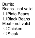
Visualizing the TreeState with a burrito ordering example
To better visualize these different nodes, let’s take a look at a burrito order in which a user can choose from two meats, chicken or steak, and two beans, pinto or black. We can take it further by allowing the user to select the quantity of meat via a nested option.
Figure 4: Ordering a burrito provides a variety of options, as displayed in the N-ary tree above, making it a helpful way to visualize an otherwise complex item.
The Burrito is an ItemNode and is also the root of TreeState. It has two child OptionListNodes, Meat and Burrito.
Beans is an OptionListNode with two child OptionNodes, Pinto and Black.
Pinto is an OptionNode.
Black is an OptionNode.
Meat is an OptionListNode with two child OptionNodes, Chicken and Steak.
Chicken is an OptionNode
Steak is an OptionNode with one child OptionListNode, Quantity, meaning it is a nested option.
Quantity is an OptionListNode with two child OptionNodes, ½ and 2x.
½ is an OptionNode
2x is an OptionNode
Class Pattern implementation on the Item Modal
We built another contrived Item Modal example on CodeSandbox to demonstrate how we use TreeState in the burrito ordering example described above. In this walkthrough, we focus on a simple example to show off the Class Pattern. However, we also include the more complicated nested options for those interested in taking a deeper dive.
We expose a useTree hook in a similar manner to how we implemented useTodo in our TodoList example above. useTree interacts with TreeState, exposing selectors for currentNode and mutation functions for selecting and unselecting options, and building the initial tree.
The first critical part to render the Item Modal is building the initial TreeState with item data, as shown in Figure 5, below.
Figure 5: In our Class Pattern flow, as shown in our Item Modal example, the first step in the cycle initializes the useTree, followed by an API call to fetch data, tree building, validation, and a final step where the tree is re-rendered.
Item Modal – We initialize the useTree hook on the initial render, exposing buildTree, currentNode, selectOption, unselectOption, setCurrentNode (not covered in this walkthrough), and addTreeNodes (also not covered in this walkthrough). When we initialize the useTree hook, the TreeState is in its default state, with currentNode undefined, root undefined, and nodeMap set to {}.
Item Modal – A useEffect hook will trigger and detect that currentNode is undefined and fetch item data and call buildTree exposed from useTree with the item data. However, in this Class Pattern example, we will omit the API call implementation and use mock data (found in TreeState/mockData).
Item API Response is received – buildTree dispatches a BUILD_TREE event to be handled by treeReducer.
treeReducer makes a deep copy of the current TreeState and then calls TreeState.handleTreeAction
TreeState.handleTreeAction begins to look a lot like a typical Redux reducer with its switch statements. In the switch statement, the incoming action type matches TreeActionType.BUILD_TREE. Here, TreeState creates all nodes, ItemNode, OptionListNode, and OptionNode, from the item data payload for the initial tree. We create ItemNode in createTreeRoot, OptionListNode in createOptionListNodes, and OptionNode in createOptionNodes.
The critical piece here is that the nodes are created with the correct pointers to their children and parents. The Burrito ItemNode’s children are Meat and Beans, which are in turn OptionListNodes with Burrito as their parent. Meat’s children are Chicken and Steak, which are also OptionNodes with Meat as their parent. Beans’ children are Pinto and Black with Beans as their parent.
TreeReducer – The initial TreeState is now updated and built, triggering a re-render in the web application component which renders the currentNode, as shown in Figure 6, below:
Figure 6: The DOM renders the Item Modal after the initial TreeState is updated and built.
After we request the item data payload, there are a lot of moving parts involved in building the initial TreeState, and a lot of places where things can go wrong. The Class Pattern allowed us to easily write tests for different types of items and check that the TreeState was built correctly.
In the example below, we write a suite of tests for our Burrito ordering use case to make sure that all the relationships and initial validity are correct between the ItemNode, OptionListNodes, and OptionNodes. We think of these as “integration” tests as they test the entire side effects of a reducer action as opposed the “unit” tests that we wrote to test the business logic of ItemNode, OptionListNode, and OptionNode. In production, we have our suite of unit tests for all types of item data payloads, such as reorder, default options, and nested options.
const treeState = new TreeState();
   treeState.handleTreeAction({
     type: TreeActionType.BUILD_TREE,
     itemNodeData,
     optionListNodeDataList: optionListData,
     optionNodeDataList: optionData
   });
   it('Burrito should be the parent of Beans and Meat and Beans and Meat should be Burrito"s children', () => {
     const burritoNode = treeState.getRoot();
     burritoNode?.getChildren().forEach((optionListNode) => {
       expect(
         optionListNode.getName() === "Meat" ||
           optionListNode.getName() === "Beans"
       ).toBeTruthy();
       expect(optionListNode.getParent()).toBe(burritoNode);
     });
   });
We have tests for all the business logic at every level of the Item Modal, covering each node level and the TreeState in the CodeSandbox below. After building a tree, we have tests that make sure that every single node is initialized correctly.
The TreeState is critical to every aspect of the Item Modal. It is involved in the Item’s Modal’s rendering, client-side validation, and data fetching. Every user interaction results in a change to the TreeState.
Rendering
With the class pattern and TreeState, the Item Modal rendering has become dead simple as we have an almost one-to-one relationship between the markup and state shapes. ItemNode renders as an Item component, OptionListNode renders an OptionList component, and OptionNode renders an Option component.
The Item Modal can be in two different states: the initial item page or on a nested option page. We won’t cover the nested option case here but we determine what type of page to render by using Type Guards.
For the initial item page, we render an ItemBody component, which accepts the currentNode, selectOption, and unselectOption as properties. ItemBody renders the name of the item, maps its children and renders OptionLists, and renders a submit button that can only be interacted with when all the options meet the correct validation criteria.
Inside ItemBody, the markup is really simple because we just render the ItemNode’s children which are OptionListNodes as OptionList components, as shown in this CodeSandbox code sample.
The OptionList component accepts optionListNode, selectOption, unselectOption, and setCurrentNode properties. Following these inputs, OptionList renders its name, determines whether the OptionListNode is valid, and maps its children, which renders Options.
The Option component accepts optionNode, selectionNode, selectOption, unselectOption, and setCurrentNode properties. selectionNode is the dynamic part of the form and determines whether a radio button or checkbox is rendered. SelectionNodeType.SINGLE_SELECT renders a radio button
The whole point of the Item Modal is to save and validate a user’s inputs and modifications to an item. We use selectOption and unselectOption functions exposed from useTree to capture these user inputs and modifications.
Figure 7: The selectOption and unselectOption functions are able to capture the user inputs in our Item Modal.
To illustrate the lifecycle of what happens when an Option’s checkbox is clicked, we will go over what happens when a user clicks the Pinto Beans checkbox from our example. The lifecycle to get to the TreeState.handleTreeAction is exactly the same as building the initial tree.
Figure 8: The TreeState is the source of truth for the Item Modal, and every user interaction dispatches an action to update the state.
Pinto Beans Clicked – handleMultiSelectOptionTouch callback is fired on onChange event. The callback checks if the OptionNode is already selected. If it is already selected, then it will call unselectOption with its ID. Otherwise, it will call selectOption with its ID.In this example, it calls selectOption.
selectOption – dispatches a TreeActionType.SELECT_OPTION action with an optionID payload.
treeReducer -deep clones the current tree state and calls TreeState.handleTreeAction.
handleTreeAction – we use getNode to retrieve the node from the nodeMap with an optionID.
case TreeActionType.SELECT_OPTION: {
      const optionNode = this.getNode(treeAction.optionId);
      if (!(optionNode instanceof OptionNode))
         throw new Error("This is not a valid option node");
       optionNode.select();
       if (optionNode.getNextCursor() !== undefined)
         this.currentNode = optionNode;
       return;
     }
OptionListNode.validate, we need to validate the user’s input and determine whether it satisfies the boundary rules set by its minNumOptions and maxNumOptions. After checking the boundary rules, the OptionListNode’s parent validate is called, which is on ItemNode.
ItemNode.validate – validation is similar to an OptionNode’s validation. It checks to see if all of its children are valid to determine if the ItemNode is valid, but it doesn’t call its parent to validate as it is the root of the tree.
Burrito – not valid, beans – valid, pinto beans – not valid – Our TreeState is updated with Pinto Beans as selected, and its parent node, Beans, and grandparent node, Burrito, have been validated. This state change triggers a re-render and the Pinto Beans option shows selected, while Beans changes from not valid to valid.
Clicking Pinto Beans works just like building the initial tree. When a user clicks an option, we need to make sure that the TreeState is updated and all of our ItemNodes, OptionListNodes, and OptionNodes are correctly set as invalid or valid. We can do the same with the initial build tree action and initialize a TreeState, fire off the select option action, then check all of the nodes to verify that everything is correct.
For any user interaction, we need to recursively climb up the tree from where the user interaction initiates, as this interaction can result in that node becoming valid and affecting its parent’s validity, and its parent’s parent’s validity, and so on.
In the Pinto Beans example, we have to validate starting from the Pinto Beans node. We first see that it does not have any children so, as a leaf node, it is immediately valid. Then we call validate on Beans because we need to check if a valid isSelected = true Pinto Beans node can fulfill our Beans boundary conditions. In this example, it does, so we flag Beans as valid and then finally we call validate on Burrito. On Burrito, we see that it has two OptionListNodes as children and Beans is now valid. However, Meat is not valid, which means Burrito is not valid, as shown in Figure 9, below:
Figure 9: For each node, pink means the node is invalid, green means that the node is valid, red means that the node was clicked and selected, and yellow means that it is validating.
How to use the Nested Options Playground
We haven’t gone through the nested options example in this code walkthrough, but the code is available in the CodeSandbox we created. To unlock the nested options example and play around with the code, please uncomment out here and here.
Conclusion
State management can get exponentially more complicated as an application’s complexity grows. As we began the migration process to microservices, we re-evaluated how data flows through our application and gave some thought on how to improve it and better serve us in the future.
The Class Pattern lets us clearly separate our data and state layer from our view layer and easily write a robust suite of unit tests to ensure reliability. After the rebuild, we leveraged the Class Pattern to build and deploy the reordering feature in late 2020. As a result, we were able to easily write unit tests to cover our new use case, making one of our most complicated features on the web into one of our most reliable.
Before, it was easy to test the entire output of an action and its side effects on the entire state but we were not able to easily get the granularity of all the moving parts (individual node validation, error messages, etc) . This granularity from the class pattern and the new ease of testing has increased our confidence in the item modal feature and we have been to build new functionality on top of it with no regressions.
It’s important as a team to find a pattern or library to commit to in order for everyone to be on the same page. For teams coping with a similar situation, where state is getting more complicated and the team is not married to a specific library, we hope this guide can spark some inspiration in building a pattern to manage the application’s state.
New service releases deployed into DoorDash’s microservice architecture immediately begin processing and serving their entire volume of production traffic. If one of those services is buggy, however, customers may have a degraded experience or the site may go down completely.
Although we currently have a traffic management solution under development for gradual service rollouts as a long-term solution, we needed an interim solution we could implement quickly.
Our short-term strategy involved developing an in-house Canary deployment process powered by a custom Kubernetes controller. Getting this solution in place gives our engineers the ability to gradually release code while monitoring for issues. With this short-term solution we were able to ensure the best possible user experience while still ramping up the speed of our development team.
The problems with our code release process
Our code release process is based on the blue-green deployment approach implemented using Argo Rollouts. This setup gives us quick rollbacks. However, the drawback is that the entire customer base is immediately exposed to new code. If there are problems with the new release, all our customers will find a degraded experience.
Our long-term answer to this problem consists of a service mesh that can provide more gradual control of the traffic flow and a special purpose deployment tool with a set of custom pipelines. This solution would allow us to release new code gradually so that any defects do not affect our entire customer base. However, this new system will take several cycles to build, which meant we needed to come up with a short-term solution to manage this problem in the meantime.
A quick overview of the blue-green deployment pattern
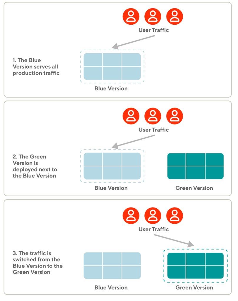
At DoorDash, we release new versions of our code following the blue-green (B/G) deployment pattern, as shown in Figure 1, below. B/G reduces the risk of downtime by keeping two versions of the same deployment running simultaneously. The blue version is stable and serves production traffic. The green version is idle and considered the new release candidate.
The actual release happens when the production traffic is switched from the blue version to the green version. After the switch, the blue version is still kept on hold as a backup in case there are problems with the green version. Rolling back to the blue version is instantaneous and immediately resolves any issues coming from the green version.
Utilizing Argo Rollouts for B/G deployments
Argo Rollouts is a framework that provides a set of enhanced deployment strategies, including B/G deployments, and is powered by a Kubernetes controller and some Kubernetes Custom Resource Definitions (CRDs). The Kubernetes objects created as part of the Argo Rollouts B/G CRD are called Rollouts. Rollouts are almost identical to Kubernetes Deployment objects, to which they add more advanced functionalities needed in scenarios such as B/G deployments.
Figure 1: The blue-green (B/G) deployment process deploys the release candidate, called the green version, alongside the stable version, called blue, which is serving all production traffic. The green version is promoted switching traffic from the blue version to the green version. The blue version is kept around idle for some time to allow for quick rollbacks.
The Argo Rollouts B/G implementation in detail
The Argo Rollouts B/G implementation is based on the Rollouts Kubernetes controller, a Kubernetes Rollout object, and two Kubernetes Services: one named Active Service and another named Preview Service. There are two separate versions of the Rollout: the blue and the green. Each version comes with a rollouts-pod-template-hash labelthat stores the (unique) hash of its specs and is computed by the controller.
The controller injects a selector into the Active Service with a value that matches the blue hash, effectively causing the Active Service to forward production traffic to the blue version. In the same way, the Preview Service can be used to target the green version in order to perform all tests needed to qualify it as production ready. Once the green version is deemed ready, the Active Service selector value is updated to match the green hash, redirecting all production traffic to the green version. The blue version is then kept idle for some time in case a rollback is needed.
The ability to almost instantaneously switch the incoming traffic from the blue version to the green version has two important consequences:
Rolling back is very fast (as long as the blue version is still around).
The traffic switch exposes the production traffic to the green version all at once. In other words, the entire user base is affected if the green version is buggy.
Our objective is a gradual release process that prevents a bug in the new release candidate code from negatively affecting the experience of our entire customer base.
A gradual deployment strategy requires a long-term effort
The overall solution to the deployment process problem we faced was to pursue a next-generation deployment platform and a traffic management system that can provide us with a more granular control of the traffic flow. However, the scope of such a workstream and the potential impact over our current setup make these changes only feasible within a time range spanning multiple quarters. In the meantime, there were many factors pushing us to find a short-term solution to improve the current process.
Why we needed to improve the current process
While our long-term strategy for gradual deployments was in the works, our systems were still at risk of disappointing all our customers at every deployment. We needed to ensure that customers, merchants, and Dashers would not be negatively affected by future outages that could erode their trust in our platform.
At the same time, our strong customer obsession pushed many of our teams towards adjusting their deployment schedules to minimize the potential customer impact of a buggy release. Late-night deployments became almost a standard practice, forcing our engineers to babysit their new production instances until early morning.
These and other motivations pushed us towards finding a short-term solution to provide our engineers with gradual deployments capabilities, without having to utilize non-optimal working requirements.
Our short-term strategy for gradual code releases: an in-house Canary solution
A Canary solution would be a fast, easy-to-build short-term solution that would allow teams to monitor gradual rollouts of their services so that buggy code would have minimal impacts and could be rolled back easily. This process involved figuring out our functional requirements, configuring our Kubernetes controller, and avoiding obstacles from Argo Rollouts.
Short-term solution requirements
We started by laying down a list of functional and non-functional requirements for our solution. It had to:
leverage native Kubernetes resources as much as possible to reduce the risk and overhead of introducing, installing, and maintaining external components
use exclusively in-house components to minimize the chance of our schedule getting delayed by factors, such as external dependencies not under our control
provide an interface that is easy to use and integrated with tools our engineers were already familiar with
provide powerful levers to control gradual deployments, but at the same time put guardrails in place to prevent potential issues like excessive stress on the Kubernetes cluster
lay out a streamlined adoption process that is quick, easy, and informed
avoid the additional risks of changing the existing deployment process, and instead integrating it as an additional step
Core idea: leverage the Kubernetes Services forwarding logic
Our solution was based on the creation of an additional Kubernetes Deployment, which we called Canary, right next to the Kubernetes Rollout running the blue version serving our production traffic. We could sync the labels of the Canary Deployment with the selectors of the Kubernetes Active Service, causing the latter to start forwarding a portion of production traffic to the Canary Deployment. That portion could be estimated starting from the fact that a Kubernetes Service load balances the incoming traffic among all the instances with labels matching its selectors. Therefore, the approximate percentage of incoming traffic hitting the Canary Deployment was determined by the following formula:
where #canary and #production represent, respectively, the number of instances belonging to the Canary Deployment and to the existing production Rollout. Our engineers can increase and decrease the number of instances in the Canary Deployment, respectively increasing and decreasing the portion of traffic served by the Canary Deployment. This solution was elegant in that it was simple and satisfied all our requirements.
The next step was to figure out how to sync the labels of the Canary Deployment with the selectors of the Active Kubernetes Service in order to implement the Canary solution.
Building a custom Kubernetes controller to power our Canary logic
One challenge to implementing our solution was to come up with a way to inject the Canary Deployment with the right labels at runtime. Our production Rollouts were always created with a predefined set of labels which we had full control over. However, there was an additional rollouts-pod-template-hash label injected by the Rollouts controller as part of the Argo Rollout B/G implementation. Therefore, we needed to retrieve the value of these labels from the Kubernetes Active Service and attach them to our Canary Deployment. Attaching the labels forces the Kubernetes Active Service to start forwarding a portion of the production traffic to the Canary Deployment. In line with the Kubernetes controller pattern, we wrote a custom Kubernetes controller to perform the label-syncing task, as shown in Figure 2, below:
Figure 2: Our custom Kubernetes controller listens to Kubernetes Events related to the creation or update of Canary Deployments. Once a matching Event is received, the controller updates the labels of the corresponding Canary Deployment so that the Kubernetes Service will start forwarding a portion of production traffic to it. This portion can be increased scaling up the Canary Deployment.
A Kubernetes controller is a component that watches the state of a Kubernetes cluster and performs changes on one or more resources when needed. The controller does so by registering itself as a listener for Kubernetes events generated by actions (create, update, delete) targeting a given Kubernetes resource (Kubernetes Pod, Kubernetes ReplicaSet, and so on). Once an event is received, the controller parses it and, based on its contents, decides whether to execute actions involving one or more resources.
The controller we wrote registered itself as a listener to create and update events involving resources of type Kubernetes pods with a canary label set to true. After an event of this kind is received, the controller takes the following actions:
unwraps the event and retrieves the pod labels
stops handling the event if a rollouts-pod-template-hash label is already present
constructs the Kubernetes Active Service name given metadata provided in the pod labels
sends a message to the Kubernetes API server asking for the specs of a Service with a matching name
retrieves the rollouts-pod-template-hash selector value from the Service specs if present
injects the rollouts-pod-template-hash value as a label to the pod
Once the design of our Canary deployment process was concluded, we were ready to put ourselves in the shoes of our customers, the DoorDash Engineering team, and make it easy for them to use.
Creating a simple but powerful process to control Canary Deployments
With the technical design finalized, we needed to think about the simplest interface that could make our Canary Deployment process easy to use for the Engineering team we serve. At DoorDash, our deployment strategy is based on the ChatOps model and is powered by a Slackbot called /ddops. Our engineers type build and deploy commands in Slack channels where multiple people can observe and contribute to the deployment process.
We created three additional /ddops commands:
canary-promote, to create a new Canary Deployment with a single instance only. This would immediately validate that the new version was starting up correctly without any entrypoint issues.
canary-scale, to grow or shrink the size of the Canary Deployment. This step provides a means to test out the new version by gradually exposing more and more customers to it.
canary-destroy, to bring down the entire Canary Deployment.
Once the interface was ready to use, we thought about how to prevent potential problems that may come up as a result of our new Canary Deployment process and build guardrails.
Introducing guardrails
During the design phase we identified a few potential issues and decided that some guardrails would need to be put in place as a prevention mechanism.
The first guardrail was a hard limit on the number of instances a Canary Deployment could be scaled to. Our Kubernetes clusters are already constantly under high stress because the B/G process effectively doubles the number of instances deployed for a given service while the deployment is in progress. Adding Canary pods would only increase this stress level, which could lead to catastrophic failures.
We looked at the number of instances in our services deployments and chose a number that would allow about 80% of services to run a Canary Deployment big enough to achieve an even split between the Canary and non-Canary traffic. We also included an override mechanism to satisfy special requests that would need more instances than we allowed.
Another guardrail we put in place prevented any overlap between a new B/G deployment and a Canary Deployment. We embedded checks into our deployment process so that a new B/G deployment could not be started if there were any Canary pods around.
Now that the new Canary Deployment process was shaping up to be both powerful and safe, we moved on to consider how to empower our engineers with enough visibility into the Canary metrics.
Canary could not exist without proper observability
Our new Canary Deployment allows our engineers to assess whether a new release of their service is ready for prime time using a portion of real-life production traffic. This qualification process is essentially a comparison between metrics coming from the blue version serving production traffic and metrics coming from the Canary Deployment running the new release candidate. Looking at the two different categories of metrics, our engineers can evaluate whether the Canary version should be scaled up further to more customer traffic or should be teared down if it’s deemed buggy.
The implementation of this observability aspect was completely in the hands of our engineers, as each service had their own naming conventions and success metrics that could vary substantially based on the nature of the service. A clear separation between Canary and non-Canary metrics was possible thanks to specific labels injected only to the Canary pods. This way, teams could just replicate the queries powering their dashboard, adding an additional filter.
We designed adoptions to be easy, quick, and informed
The next and final step was to plan for helping the Engineering team adopt the Canary Deployments. As always, our objective was a quick and painless adoption. At the same time, we were providing our engineers with a powerful tool that was using our production traffic as a testbed, so we needed them to be empowered with knowledge about potential pitfalls and how to act in case things went wrong.
To onboard engineers quickly and safely, we designed a four-step adoption process that they could follow without any external help, as it was simply re-using concepts they were already familiar with. In this case we tried to stay away from fully automating the adoption process as we wanted them to understand its details. We also added a validation step at the end of the process that required explicit approval. This validation step enabled us to sit down with first-time users and guide them through their first Canary Deployment, explaining what was happening under the hood and what to do in case of failure.
The adoption campaign went better than anticipated
Initially, we prioritized adoptions for about a dozen services on the golden path of our workflows. Reducing the chances of those services suffering from a full outage meant improving by a great deal the reliability of the core customer flows that power our business.
We had a lot of positive feedback about the adoption procedure and the new Canary process overall, and what we observed was that additional teams onboarded their services and scheduled time with us to review their configuration. We ended up onboarding about twice the number of services we anticipated before the end of the year, which was a huge success, taking into account a deploy freeze during the holiday season.
Conclusion
Releasing new code carries risk and associated costs that can be mitigated using a gradual rollout strategy. However, Kubernetes does not provide this capability out of the box. All the existing solutions require some form of traffic management strategy, which involves significant changes at the infrastructure level and an engineering effort that can last multiple quarters.
On the other hand, the Kubernetes controller pattern is a simple but extremely powerful technique that can be used to implement custom behavior for Kubernetes resources, like advanced deployment strategies.
Thanks to our new Canary Deployment process powered by a custom Kubernetes controller and other company-wide efforts towards improving the reliability of DoorDash services, our customers, merchants, and Dashers can put their trust in our platform while our engineers work with greater velocity.
The author would like to thank Adam Rogal, Ivar Lazzaro, Luigi Tagliamonte, Matt Ranney, Sebastian Yates, and Stephen Chu for their advice and support during this project.
The technical interview, is a crucial component of the interview loop for software engineers, that gauges the candidate’s ability to perform in the role under consideration. The skills required to successfully complete a technical interview at DoorDash include demonstrable knowledge in data structures and algorithms, and the ability to effectively communicate and problem solve.
Typically, an experienced engineer takes the role of interviewer, assessing the candidate’s strengths and weaknesses. While the technical interview may seem challenging, it’s important to remember that the interviewer’s honest goal is to find someone who can be a great contributor to a team working on projects that fulfill the company’s business goals.
As a member of a small team of engineers here at DoorDash who contribute to and vet the questions asked in our technical interviews, as well as an active interviewer, I’ll highlight some key pieces of our technical interview. Ultimately, we want excellent candidates who succeed in every part of our interview loop, find a place at DoorDash, and build a highly satisfying career.
Background
Interviews are an attempt to make the best of a difficult situation. In a few short hours we need to figure out if a candidate can successfully contribute to their team and the company over what might end up being many years. As Lokesh Bisht, the Director of our Customer Analytics team, pointed out in his article on the data science interview, the technical interview is a means to mitigate the cost of bad hires by taking a snapshot of some of the candidate’s skills. Our interview questions need to be well-considered to give an unbiased assessment.
Interviewers can have different styles and expectations on what they expect to see in a successful candidate. By highlighting the general structure and process of our technical interview, we want to give candidates the best possible preparation for success.
Data structures and algorithms
Many tech companies stack their interviews with questions related to specific algorithms and data structures, and DoorDash is no different. Candidates should feel comfortable using, as well as understanding, the key differences and applications of the following data structures:
This list doesn’t imply other data structures won’t be included in the interview, it just means the ones listed above tend to be more commonly covered. I also highly recommend candidates be well-versed with the worst, best, and average runtime complexities for inserting, removing, and finding elements in all data structures they feel comfortable using.
Candidates should also be well-versed in the following algorithms:
Common sorting algorithms (merge, insert, bubble, etc) -> not expected to memorize, but understanding when to use them is recommended
Binary search
General comfort in complex searches and sorts in above data structures
Stay Informed with Weekly Updates
Subscribe to our Engineering blog to get regular updates on all the coolest projects our team is working on
Please enter a valid email address.
Thank you for Subscribing!
Communication
The concept of having a communicative approach to solving problems isn’t always emphasized in academic settings. However, we use communication as a metric in determining the success of a candidate due to the importance of teamwork in our engineering organization. Below are some key points to keep in mind.
Keep the interviewer involved
Ideally, we want the candidate to complete the problem and all associated subproblems successfully without any help from the interviewer. However, we encourage candidates to keep the interviewer informed about what they are trying to accomplish. There’s no need for a constant, ongoing conversation, but it is important to describe key decision steps while answering a question.
Here are some examples:
“We can use a stack for this solution because…”
“We can use an in-order tree traversal for this question because…”
“I may have missed some edge cases, let me take a closer look at my solution.”
“I can think of a solution in O(N2) time doing X, but I think we can have a linear solution here. I’d like to take a minute to think through an approach.”
I wouldn’t expect a candidate to talk while coding or pseudocoding their solution (in fact, I find it hard to think and talk at the same time, so I prefer silence during those parts of the interview). Candidates should take time to collect their thoughts, but make sure the interviewer is following the process at key points, such as:
Clarifying questions after being given the problem
The approach to solving the problem
Identifying potential flaws in the approach
Changing direction to a new approach
The interviewer is there to gently guide the candidate to a final solution and to help them score the most points possible for that candidate’s knowledge and skill base.
It’s okay to think
Far too often technical interview tutorials and guides suggest that interviews consider long moments of silence as a negative, and can lead to losing points. There is absolutely nothing wrong with taking time to think about the interview question and in constructing a coherent solution. I’d encourage candidates to take a one or two minute pause in situations which warrant critical thinking.
Feedback
Don’t expect constant feedback when solving a problem. An interviewer’s job is to help candidates stay on course toward a working solution, but only if they need it. Generally, candidates will lose points if the interviewer needs to steer them back towards a solution or give them large hints on something they missed. We train our interviewers to only step in when they believe the candidate has a higher chance of scoring better with their intervention.
Solving the question
Regardless of a candidate’s approach to solving technical interview questions, there are some steps that should usually be taken.
Remove ambiguity
DoorDash engineers often find themselves solving questions with many unknowns and few clear paths to move forward. The interview process helps us assess this skill in candidates, which is needed to be successful here. We often make questions ambiguous on purpose, and it is the candidate’s responsibility to remove any ambiguity. A candidate may miss edge cases if they don’t clarify the problem.
In this linked example question, there are a few constraints specifically left out of the question description. If they aren’t accounted for in the solution, there may be some edge cases missed, resulting in a lower score.
Brute force
In general I advise not to go with a brute force approach as a final solution. In every case where there is an optimal solution with significant complexity improvement, a typical brute force solution will result in a low score for the problem.
Constructing a solution
A perfect solution doesn’t need to be achieved instantly. Take some time to come up with a general approach and iterate on top of it until it works. I recommend creating a working solution and then running through a test case with the interviewer to find any bugs. We highly value debugging skills, and candidates won’t lose any points if they are able to find their own mistakes and rectify them without interviewer intervention. After coming up with a good solution, candidates can move forward with runtime analysis and follow-up questions (which are very common in our interviews).
Runtime analysis
Candidates should have a strong understanding of runtime and in-memory complexities for their approach. In general, candidates should be able to clearly explain every step of the solution and why they chose the approach. For example, why use a linked list in a solution instead of an array?
Unit testing
Although not expected for all questions, some questions will ask candidates to write their own unit tests. Be aware of industry standard testing practices and be able to construct meaningful, yet concise unit tests. Show clear thought and understanding in each unit test, avoiding repetition while still giving confidence to the solution.
I recommend books such as Clean Code and Code Complete 2 for theoretical knowledge on unit tests as well as other standard software engineering practices.
Preparation
Preparation is key to tackling the technical interview. The ideal situation for candidates is to find themselves solving a problem very similar to problems they previously solved.
Consider the following resources:
Data structure/algorithms practice tools, such as LeetCode
One-on-one interview preparation tools, such as interviewing.io
A great way to prepare for the technical interview involves practicing with a friend and on a whiteboard or remotely using a shared screen. Working out a sample problem in this manner will make the actual interview situation more familiar.
Scoring
In addition to the general success of solving the questions asked, there are three main categories considered when assessing a candidate’s success:
Fundamentals
Understands common data structures and when to apply them
Can perform time and space complexity analysis
Arrives at correct and optimal (in time and space) solution
Coding
Thinks about good abstractions for solving the problem at hand
Writes well-organized code, with correct syntax, in their language of choice (there is no point difference for choice of language)
Effectively tests and debugs code
Communication
Asks clarifying questions to eliminate ambiguity
Explains their thought process when coming up with a solution
Receives feedback well, without getting overly defensive
Other interviews
While the above focuses on the algorithm/data structure portion of our technical interview, there are other modules of our interview loop. Which modules a candidate encounters depends on the nature and seniority level of the role the candidate is being interviewed for.
Values
This part of the interview assesses whether a candidate can exemplify our DoorDash values, such as exhibiting a bias for action, getting 1% better every day, and making room at the table. Every candidate goes through this interview, which involves general questions about past challenges and successes, how they would cope with certain theoretical situations, and their career intentions. The candidate will also be afforded the opportunity to ask questions at the end of this interview to assess whether DoorDash feels like a place where they can do some of the best work of their career.
System design
The system design interview is typically given to industry-level, as opposed to entry-level, candidates (L4-plus), and can be a major tool in assessing the candidate’s skill level. It is generally a more difficult interview to practice for. The question assesses a candidate’s ability to build a scalable system with well-thought-out design decisions. These questions are often left intentionally vague and use a real setting. This interview usually gives a deep-dive into one or two specific pieces of the design while taking a shallower glance at the other pieces.
To prepare, candidates are encouraged to research and reverse engineer common systems within their domain. Frontend candidates, for example, can practice using popular applications such as Gmail or DoorDash. Backend engineers can deep dive into specific areas within large systems such as Twitter or a messenger service.
Backend
The backend system design question is often grouped together with domain knowledge, but may also be separated into two rounds depending on which team has the open role. Chao Li, a backend engineer on our Ads and Promotions team, shares his thoughts below:
“This interview usually focuses on a couple of areas, with increased difficulty levels:
The first part, which most candidates can get through with little difficulty, involves a breakdown of the problem requirements and suggesting basic components. This area requires steps such as understanding the problem statement, translating requirements into technical components, breaking down the data model, suggesting an API, and coming up with a database schema.
Candidates should be prepared to dive deep into each component and talk about how different situations are handled. Typical examples include how a payment component handles double writes, or how a distributed queue handles surges and failures.
Be ready to discuss details about their approach. For example, if a candidate mentioned using a message queue to solve the problem, we would expect justification for why a message queue is the best solution, what are the trade-offs for the specific product versus other products (i.e., AWS Kinesis over an on-premises Kafka cluster), what were some other potential solutions, what are the pros and cons, and what are the failure scenarios for this solution.
The last part of this interview concerns scalability. We assess whether a candidate knows how to get from zero to a 1x solution, as well as a 1x to a 10x solution. In particular, the candidate should be able to suggest how the tech stack and architecture will need to evolve to achieve scale.“
iOS
The iOS interview, commonly referred to as the architecture interview, will dive into application design, which will later be implemented in a coding round. Tom Taylor, an engineer on DoorDash’s iOS platform team, shares his thoughts below:
“During the architectural interview, candidates are given a feature and design and expected to whiteboard an iOS system. No coding is required for this interview; we mainly talk about elements at a class, struct, or interface level. While we do not require every candidate to be expert software architects, it is important when designing a feature to consider testing, scalability, data flow, and techniques for managing code when working on a larger codebase. Also, candidates should understand how to design a system without relying on third-party libraries.”
Android
The Android interview usually involves a dedicated portion to go over system design. As preparation, we recommend going through some common apps and being able to give a deep dive into, or reverse engineer, them. The question may not be to design an app doing a specific task, but could also involve designing a library that an app may use. For example, candidates may be asked to design an image loading library similar to Glide.
It’s important to have strong fundamentals, such as threading, caching, memory and battery consumption, network usage, scalability, app persistence, and interaction with the operating system to succeed in this interview.
Web
This interview will typically go through developing a web application. Michael Sitter, tech lead for DoorDash’s Web Platform team, shares his thoughts below:
“We don’t expect candidates to necessarily be able to describe solutions for scalability and fault tolerance, but the best candidates are able to include those qualities in their designs. Instead, we try to focus on things like the contracts between the web/client applications and the backend APIs. What data do we need to collect? How should the client app respond to various API responses? Synchronous or asynchronous? How do we handle cases where we have high or low latency?”
“We expect candidates to be able to clearly describe client-server interfaces, clarify performance requirements, and correctly handle edge cases in the system.”
Domain knowledge
The domain knowledge interviews test the candidate’s fundamentals in the platform they are applying for. They should be comfortable with basic terminology and applications within the given domain as well as demonstrate a strong understanding of the infrastructure they are using. This interview involves a deep dive into an example project in the domain area. We usually conduct this interview in a question-and-answer format, and it is occasionally combined with the system design interview. iOS candidates normally don’t go through this interview in their loop, as it is replaced with a debugging round explained in the Coding section below.
Coding
Some interview loops contain a coding round. This module usually follows a take-home project involving a real-world application and will ask the candidate to add or change a feature within their already built application. This interview is used to assess a candidate’s proficiency in the language and platform they are working in as well as how they architect their code.
iOS Coding
The iOS interview loop differs slightly from other platforms. Candidates will forgo the domain knowledge and coding interviews described above and instead go through two modified coding rounds. In the first round, the candidate will implement the design they have built in the system design/architecture interview. During the second round, they will receive an application in xCode with some errors and flaws, and are expected to debug the codebase into a working solution.
There is also no take-home project during iOS interviews. Instead, we ask candidates to participate in a technical phone screen where they will work with an iOS engineer in finishing a partially completed application. This module is done prior to any on-site interviews.
Conclusion
Interviewing can be an unnerving and sometimes challenging experience, but it gets much easier through repetition and practice. Along with a skill evaluation, however, candidates also get a chance to see how their prospective colleagues think and communicate as well as a glimpse into the types of problems we solve at DoorDash.
I hope to provide ample preparation materials in order to mitigate against some of the biases that come with interviewing and to let the process highlight the prospective connection between the interviewee and the company. I wish nothing but success to any future candidates and I hope we can be a great environment for candidates to advance their careers.
If you are interested in building a logistics platform that supports local economies, consider joining our team!
When companies move to microservices, they need to address a new challenge of setting up distributed tracing to identify availability or performance issues throughout the platform. While various tools offered on the market or through open-source perform this task, there is often a lack of standardization, making leveraging these tools costly or complicated.
As DoorDash migrated off its monolith to microservices, we considered these issues and chose OpenTelemetry, an open source distributed tracing project, for its emphasis on telemetry data standardization. To make this implementation successful, we needed to ensure that we could utilize OpenTelemetry without incurring any performance costs that would negatively affect our platform and user experience. To do this, we created a baseline of how OpenTelemetry performed on our platform. We then researched six ways of optimizing its performance and compared them side by side to pick a winner.
What is distributed tracing?
Before we jump into our benchmarking experiments, let’s review some important terminology. Tracing is the process of specialized logging that records information about a program’s execution in real-time. A trace, for example, contains information about the time a program spends in a function. Traces are generally helpful in debugging software performance issues.
Tracing in a monolith architecture is relatively easy. But in a microservice architecture, where a request travels through many services, it is often difficult to get an end-to-end picture of the request’s execution, making it challenging to identify availability or performance issues through traditional tracing.
Distributed tracing, a method to profile and monitor applications built on microservice architecture, solves traditional tracing challenges. As DoorDash moved away from a monolith architecture to a microservice distributed architecture, we needed distributed tracing to identify and resolve availability and performance issues quickly.
Many open source projects or commercial vendors provide distributed tracing. However, for many of the options on the market, there is a lack of standardization, resulting in a lack of data portability and a costly burden on users to maintain the distributed tracing instrumentation libraries. The OpenTelemetry project solves the standardization problems by providing a single, vendor-agnostic solution.
What is OpenTelemetry?
OpenTelemetry is a collection of tools, APIs, and SDKs to instrument, generate, collect, and export metrics, logs, and traces for analysis to understand software’s performance and behavior. OpenTelemetry formed as a merger of OpenTracing and OpenCensus after the developers of those projects decided that it’s better to develop a single, vendor-agnostic approach for enabling observability.
OpenTelemetry supports three data sources: traces, metrics, and logs. At Doordash, we decided to adopt OpenTelemetry for traces and began testing its distributed tracing feature for our platform.
How does distributed tracing work using OpenTelemetry?
Once we decided to use OpenTelemetry, we wanted to look into its distributed tracing functionality. Distributed tracing tracks a single request’s progression across the multiple services that form an application. An example of a request might be a call from a mobile endpoint or a UI action by an end-user. A single trace is essentially a tree of spans, where spans are objects that represent a unit of work done by individual services or components involved in the request. A single trace contains a single root span that encapsulates the entire request. The root span would contain child spans which in turn may have child spans.
Using OpenTelemetry, services generate a trace with a globally unique identifier. OpenTelemetry propagates the trace context to all underlying services where each service generates the spans. OpenTelemetry sends the spans to a local collector, which enhances the trace data with custom metadata. The local collectors send the trace data to a collector gateway, where they are processed and shipped to distributed tracing tools such as Jaeger, NewRelic, Splunk or LightStep for storage and visualization.
The trace identifier generated at the root span remains the same for all the child spans within the request. Distributed trace visualizers use this trace identifier to stitch together the spans generated for the same request, thus providing an end-to-end picture of the request execution across the application. Figure 1, below, outlines the high-level architecture of how we set up OpenTelemetry’s distributed tracing.
Figure 1: OpenTelemetry handles the spans generated by microservices and exports them to a local collector. The local collector enhances the trace data with custom metadata and sends them to a collector gateway. The collector gateway processes the trace data and exports it to tracing tools for storage and visualization.
Load testing OpenTelemetry to identify performance impact
Any significant increase in request latency or CPU overhead would mean a negative experience for DoorDash users or higher resource usage. Once we decided to adopt OpenTelemetry, we wanted to understand the performance impact of using OpenTelemetry’s distributed tracing functionality in our services.
Using our internal load testing tool, we tested the OpenTelemetry agent attached to a NettygRPC service written in Kotlin. The gRPC service has two rpc calls, createMessage and getMessages, which use AWS’ simple queue service to store and retrieve the messages. OpenTelemetry’s Java agent is attached to the service with the following span exporter configuration options:
We hit the two rpc calls using a synthetic load generating ~500 peak rps. The service deployment has a 1000 millicores CPU and 1000 mebibytes memory allotted in a Kubernetes cluster. We observed 72% pod CPU utilization at peak but only observed 56% pod CPU utilization at peak without the exporter. These experiments show that we have to spend more computing resources to adopt OpenTelemetry in our platform.
Figure 2: We observed 56% pod CPU utilization when OpenTelemetry’s exporter is disabled Figure 3: We observed 72% pod CPU utilization when OpenTelemetry’s exporter is enabled. The CPU utilization is higher compared to the experiment where the exporter is disabled
At this point, we noticed an increase in CPU usage with OpenTelemetry when the span exporter is enabled. CPU profiling is generally helpful in identifying these kinds of problems. Our internal load testing tool has an option to enable the YourKit Java profiler and automatically collect CPU profiling data from the service under test. We leveraged this profiling option to collect the CPU profiling data to identify the performance issue. The CPU profiling data showed a background thread named BatchSpanProcessor_WorkerThread that is continuously polling spans from a blocking queue.
Figure 4: Profiling stack traces show the CPU overhead is coming from the batch span processor’s worker thread
Note that even though the profiler shows that the batch span processor’s thread is in a waiting state, there is a direct and indirect CPU cost due to the kernel’s context switches. We played with the batch span processor’s (BSP) options as described below to see if they would help reduce the CPU overhead, but they didn’t help.
Increased batch size otel.bsp.max.export.batch.size to 5120
Reduced trace sampling otel.traces.sampler.arg to 0.01
Increased schedule delay otel.bsp.schedule.delay to 300000 (5 minutes)
Once the workarounds discussed above didn’t help resolve the performance problem, we wanted to do a deep dive into the implementation of OpenTelemetry’s BSP.
How does OpenTelemetry’s BSP work?
Once we identified that the BSP is causing the CPU overhead, we inspected OpenTelemetry’s codebase and its configuration options to understand BSP. Figure 5, below, shows the implementation of BSP, the component in OpenTelemetry that processes the spans generated by microservices and exports them to the collector.
Figure 5: Service threads add spans to a bounded blocking queue. Exporter thread polls the queue continuously and sends the spans to the collector in batches
otel.bsp.max.queue.size controls the maximum number of spans in the waiting queue. Any new spans are simply dropped once the queue is full.
The exporter thread waits until the current number of spans it collected from the queue reaches otel.bsp.max.export.batch.size before sending them to the collector in one batch. Batching, as explained above, makes perfect sense to reduce the overhead of any network or I/O calls.
Once every otel.bsp.schedule.delay interval, the exporter thread will send any spans it collected from the queue.
Creating benchmarks to establish a performance baseline for the BSP
After going through the BSP’s implementation, we noticed two apparent issues. The first one is the lock contention with the ArrayBlockingQueue. ArrayBlockingQueue uses an exclusive lock to provide threads safe access to the underlying queue. Only one thread holds access to the queue at a time while other threads wait for their turn. This access pattern results in threads doing a lot of waiting, leading to low throughput.
The second issue is the exporter thread’s continuous polling. The exporter thread receives a signal for each new queue entry due to the continuous polling, which causes context switch overhead resulting in high CPU usage. We wrote two benchmarks using Java Microbenchmark Harness (JMH) that surfaced the above two performance issues, then we established a performance baseline and compared the new BSP’s implementations.
Use Java Microbenchmark Harness to write benchmarks
Writing benchmarks using a naive framework is difficult and gives misleading results as many JVM and hardware-level optimizations are applied to the component under test, making the code appear to perform better than in reality. These optimizations are not applicable when the component under test runs as part of a larger application. JMH provides a convenient way to warm up JVM, run multiple iterations, and create multiple worker threads.
The example shown below runs a benchmark measuring throughput (operations per second) with five threads, warms up the JVM for a second, and runs five iterations where each iteration runs for five seconds. Each thread continuously processes a new span for the entire duration of the benchmark.
Establishing the right metrics for performance comparison
Once we decided to use JMH to write benchmarks, we wanted to establish the right performance metrics to compare the BSP’s different implementations.
The number of span exports per second
Although the primary JMH metric, operations per second, is a good metric in general, the number of spans getting exported is much better for understanding the BSP’s performance and effectiveness. For example, an implementation of the BSP that aggressively drops the spans would have very high throughput, but it does little valuable work because traces have missing spans. JMH provides a convenient way to track secondary metrics such as exports per second. We will be using the metric exports per second going forward to compare different versions of the BSP. Since we are interested in testing BSP in an isolated environment, we faked the network calls that send spans to the collector to do nothing. This kind of faking was necessary to prevent any external noise in the benchmark experiments.
Measuring CPU time of the exporter thread
Measuring CPU usage of the exporter thread is also very important since we are interested in making the exporter thread very lightweight. Measuring exporter thread CPU is very tricky with JMH since it consumes as much CPU as possible to hit peak throughput. We employed a simple hack shown in the example below to run the benchmark in a steady state. Adding a significant sleep in the JMH worker threads, we generated consistent requests per second.
private static void doWork(BenchmarkState benchmarkState) {
 benchmarkState.processor.onEnd(
     (ReadableSpan) benchmarkState.tracer.spanBuilder("span").startSpan());
 // This sleep is essential to maintain a steady state of the benchmark run
 // by generating 10k spans per second per thread. Without this, JMH outer
 // loop consumes as much CPU as possible making comparing different
 // processor versions difficult.
 // Note that time spent outside of the sleep is negligible allowing this sleep
 // to control span generation rate. Here we get close to 1 / 100_000 = 10K spans
 // generated per second.
 LockSupport.parkNanos(100_000);
}
While running the benchmark, we used the YourKit Java profiler to measure the CPU time of the exporter thread.
Configuration used for the benchmark
All the benchmark experiments are using the configuration given below.
otel.bsp.max.queue.size = 2048
otel.bsp.max.export.batch.size = 512
otel.bsp.schedule.delay = 5000ms
Benchmark results with different implementations of the BSP
Once we established the metrics, it was easy to compare and contrast the BSP’s different implementations. The goal is to increase the exports per second while reducing the CPU usage of the exporter thread. We will be using throughput to signify the exports per second in the benchmark results. Note that all the benchmark results discussed below are from runs using a 2.4 GHz 8-core Intel processor. When trying to figure out the best batch span processor, we looked at the following options:
For each of these options, we ran the benchmarks and compared the results. This approach gave us a side-by-side comparison of exports per second and the CPU time, which enabled us to pick a winner and use it in OpenTelemetry’s BSP.
BSP using ArrayBlockingQueue
The implementation using Java’s inbuilt ArrayBlockingQueue is the existing implementation and was used as a baseline. It uses a preallocated array buffer to implement the queue and a lock for concurrent access. Figure 6 and Figure 7, below, show the benchmark results while using this approach.
Figure 6: We can see a massive drop in throughput with an increase in the number of threads due to lock contention with the array blocking queue.Figure 7: There is a significant increase in CPU time with an increase in the number of threads due to lock contention and constant polling of the queue.
Our benchmark results show that the ArrayBlockingQueue approach does not scale since the throughput and CPU time get steadily worse as the number of threads increases mainly due to the lock contention.
There is additional overhead hurting the throughput besides the lock contention with the increasing number of threads. A rising number of threads usually puts pressure on the memory subsystem, resulting in decreased performance. Modern processors rely heavily on cache memory to keep a thread’s state. Cache memory is usually one or two orders of magnitude faster than main memory. When we have too many threads, the cache becomes full, and the processor has to evict the cache entries frequently. The evictions result in frequent cache misses leading to main memory access, resulting in decreased performance.
BSP using ConcurrentLinkedQueue
The next obvious choice is to use Java’s inbuilt ConcurrentLinkedQueue. ConcurrentLinkedQueue implements a non-blocking algorithm using atomic compare-and-swap (CAS) supported by modern processors. Given the nature of the algorithm, it is only applicable to an unbounded queue. An unbounded queue is not a great option since we need to allocate memory for every push operation with the queue and deallocate once the entries pop from the queue head. Figure 8 and Figure 9, below, show the benchmark results we got while using this approach.
Figure 8: There is a significant increase in throughput due to less lock contention, but the throughput flattened out early with an increase in the number of threads.Figure 9: There is a visible decrease in CPU time but a quite significant overhead remains
Using ConcurrentLinkedQueue, we see an increase in throughput and a decent decrease in the CPU time of the exporter thread. However, the throughput flattens out much earlier than expected with the increase in the number of threads. We identified that there are subtle issues with concurrency on a queue data structure.
We noticed that there is contention on head or tail even with CAS. The head and tail usually occupy the same cache lines, making cache coherence very expensive in modern processors due to frequent cache misses. This performance degradation phenomenon is commonly known as false sharing.
size() implementation of ConcurrentLinkedQueue is actually linear in complexity. Since OpenTelemetry specifications require a bounded size queue, we had to use an atomic counter to efficiently track the queue size and find whether the queue is full.
BSP using LMAX Disruptor
LMAX Disruptor, our next choice, is designed to address the concurrency concerns with queues. The key design ideas used by the Disruptor are:
It uses sequencing, a concurrency technique, to reduce lock contention with multiple producers. Producers claim the next slot in the ring buffer using an atomic counter. The claiming producer updates the ring buffer’s entry and commits the change by updating the ring buffer’s cursor. The cursor represents the latest entry available for consumers to read.
Consumers read from the ring buffer and have different waiting strategies when waiting for new entries.
Once we picked the Disruptor, we proceeded to the benchmark experiments with the two most common waiting strategies offered by Disruptor, TimeoutBlockingWait and SleepingWait.
Disruptor using TimeoutBlockingWait strategy
We first tried out the Disruptor with the timeout blocking wait strategy. When using this waiting strategy, the Disruptor lets consumers wait for new entries in the ring buffer using a conditional variable. This waiting strategy is similar to how the exporter thread is waiting for new entries using ArrayBlockingQueue or ConcurrentLinkedQueue. Figure 10 and Figure 11, below, show the benchmark results we got while using this approach.
Figure 10: The benchmark results show a very similar throughput to ConcurrentLinkedQueue, except we see less contention and an improved throughput with 20 threads Figure 11: The benchmark results show a very similar CPU time to ConcurrentLinkedQueue, which is what we expected given that this waiting strategy is the same as the one we implemented using ConcurrentLinkedQueue.
The benchmark results show that the Disruptor with TimeOutBlockingWait strategy is a good choice because of the increase in throughput and decrease in CPU time compared to the baseline. These improvements occur because of the Disruptor’s non-blocking algorithm. The benchmark results also show that this approach did not perform better than the ConcurrentLinkedQueue approach, revealing that the writer threads’ signaling was the bottleneck.
Disruptor using SleepingWait strategy
After using the timeout blocking wait strategy, we wanted to try out the Disruptor with the sleeping wait strategy. When using this wait technique, the Disruptor’s consumer threads that are waiting for new entries initially go through a busy-wait, then use a thread yield, and eventually sleep. According to the Disruptor documentation, this waiting strategy will reduce the producing thread’s impact as it will not need to signal any conditional variables to wake up the exporter thread. Figure 12 and Figure 13, below, show the benchmark results we got while using this approach.
Figure 12: The benchmark results show a vast improvement in throughput. A near zero contention on the write path with no signaling overhead and a busy-wait on the exporter thread contributed to this improvement. But the busy-wait wastes CPU cycles, we could see its impact in the throughput drop with 20 threads. Figure 13: The benchmark results show a huge increase in CPU time due to busy wait of the disruptor’s sleeping strategy. This high CPU time makes this approach not viable.
The benchmark results show that the Disruptor with SleepingWait strategy is not a good choice because of the significant increase in CPU time compared to the previous approaches. We noticed that this increase in CPU time was due to the busy-wait of the exporter thread. It is important to note that the benchmark results show that this approach was better for high throughput. This high throughput occurred because this approach did not require signaling of the exporter thread. However, the throughput flattened out with 10 threads or more due to the pressure on the memory subsystem and the CPU cycles wasted by the busy-wait. After analyzing these benchmark results, we moved to explore new ways of reducing the signaling overhead while lowering the exporter thread’s CPU time.
Batching the signals to reduce the exporter thread’s CPU time
Thus far, the benchmarks with different implementations showed us the most significant bottleneck to throughput is the writer threads’ locking and signaling, and the significant CPU cost to the exporter thread is context switching or a busy-wait.
The exporter thread is notified about any new entry right away, even though it will export the spans only when its buffer reaches maximum export size. This kind of exporting behavior allows us to reduce the exporter’s thread CPU time by notifying only when it will end up doing the export operation.
We use an atomic integer to let the writer threads know the number of spans the exporter thread needs for the export operation. The hypothesis is that this kind of signal batching will reduce the writer threads’ contention and the exporter thread’s frequent context switches. Below is a pseudocode implementation of the signal batching.
// pseudocode of the writer thread
if queue.offer(span):
 if queue.size() >= spansNeeded.get():
   // notify the exporter thread
   signalExporterThread()
// pseudocode of the exporter thread
while continue:
  while queue.isNotEmpty() and buffer.size() < EXPORT_SIZE:
    // Fill the local buffer
    buffer.add(queue.poll())

  if buffer.size() >= EXPORT_SIZE:
    // Export the buffer
    export(buffer)

  if queue.isEmpty():
    // Wait till there are enough spans for next export
    spansNeeded.set(EXPORT_SIZE - buffer.size())
    waitForSignal(WAIT_TIME)
    spansNeeded.set(Integer.MAX_VALUE)
BSP using signal batching and ArrayBlockingQueue
This implementation uses the ArrayBlockingQueue but batches the signals. Figure 14 and Figure 15, below, show the benchmark results using this approach.
Figure 14: The benchmark results show a very good improvement in throughput with signal batching compared to batch span processor’s implementation without signal batching. But the throughput suffered due to lock contention with the blocking queue. Figure 15: The benchmark results show a huge decrease in CPU time of the exporter thread. This confirms the hypothesis that signal batching would reduce the exporter thread’s context switches.
The benchmark results show that the signal batching with ArrayBlockingQueue is a good choice compared to the baseline because of the improvement in throughput and a significant decrease in the CPU time. But, the throughput suffered with the increase in number of threads due to lock contention and pressure on the memory subsystem. We therefore proceeded to test signal batching with other queue implementations.
BSP using signal batching and ConcurrentLinkedQueue
This implementation uses Java’s inbuilt concurrent linked queue to reduce lock contention and signal batching to reduce the exporter thread’s CPU time. Figure 16 and Figure 17, below, show the benchmark results using this approach.
Figure 16: The benchmark results show a huge improvement in throughput due to reduced contention but throughput flattened out early similar to the ConcurrentLinkedQueue implementation without signal batching. Figure 17: The benchmark results show a similar CPU time of the exporter thread with BlockingQueue and signal batching.
The benchmark results show that the signal batching with ConcurrentLinkedQueue is a good choice compared to the previous approaches because of the improvement in throughput and significant decrease in the CPU time. We then proceeded to test signal batching with other queue implementations to see if we could find an even better solution.
BSP using signal batching and disruptor
The LMAX Disruptor doesn’t offer any batch waiting strategy. Although it is possible to implement a new waiting strategy inside the Disruptor, we found an alternate solution, described in the next section, that is much easier to implement.
BSP using signal batching and MpscQueue
Even though LMAX Disruptor is not applicable with regard to batching signals, the Disruptor’s fundamental design principles, as shown in the above benchmarks, worked very well to mitigate the concurrent linked queue’s contention issues. We learned about different concurrent queue implementations offered by the JCTools library, and the multi-producer single consumer queue (MpscQueue) worked perfectly for the BSP’s use case.
It is tailor-made for the BSP’s use case where we have multi-writer threads and a single consumer, the exporter thread.
It uses a ring buffer and sequencing to resolve head or tail contention. The preallocated ring buffer implies there is no unnecessary garbage collector activity.
MpscQueue doesn’t signal the consumer about the new entries, so it is easy to implement custom signaling with batching.
We noticed that MpscQueue is very similar to the Disruptor, but we can easily apply the signal batching. Figure 18 and Figure 19, below, show the benchmark results using this approach.
Figure 18: The benchmark results show this approach to be the best performer. MPSCQueue reduces the write contention seen with the ConcurrentLinkedQueue implementation and signal batching reduces the overhead of notifying exporter thread and context switches. The throughput flattened out with ten worker threads due to the pressure on the memory subsystem similar to what we have seen in other benchmark results.Figure 19: The benchmark results show this approach to be the best performer. MPSCQueue with signal batching has reduced the CPU time of the exporter thread even more than using signal batching with other queue structures.
The benchmarks show that MpscQueue with the signal batching approach is best for high throughput and a less CPU intensive batch span processor. MpscQueue does resolve the write contention issue seen in ConcurrentLinkedQueue and, with signal batching, reduces the CPU overhead of the exporter thread. The throughput flattened out with ten threads or more due to the pressure on the memory subsystem as seen in the previous benchmarks. We learned that the existing waiting strategies with the Disruptor tend towards lowering the latency and are CPU intensive, whereas MpscQueue with signal batching proved to be a good alternative.
And finally, the load test that initially revealed the problem showed us the optimization reduced CPU utilization.
Figure 20: We observed 56% pod CPU utilization when Open Telemetry’s exporter is disabled. Figure 21: We observed 56% pod CPU utilization when Open Telemetry’s exporter with the new batch span processor is enabled. The experiment showed that the optimizations helped reduce resource usage.
Trade-Offs with signal batching
Although MpscQueue with signal batching worked best with the default configuration options, it hurts throughput if the export batch size (otel.bsp.max.export.size) is close to the maximum queue size (otel.bsp.max.queue.size) or higher. The trade-off for higher throughput is using a bigger queue with a size greater than the export batch size.
Conclusion
For any companies running on a microservice architecture, distributed tracing is an essential tool. OpenTelemetry is an excellent choice for addressing distributed tracing needs, but the performance issues we have seen with OpenTelemetry’s BSP component could negatively impact throughput and increase resource usage costs.
To address the negative impact, we contributed benchmarks and fixes to the OpenTelemetry project. Specifically, we contributed JMH benchmarks and optimizations in the BSP to improve throughput and reduce CPU cost. These optimizations will be available in the next release of the OpenTelemetry java library. Generally speaking, we believe the benchmarks and the different queue implementations we discussed could be applied to build highly performant multi-threaded producer-consumer components.
Acknowledgments
Thanks to Amit Gud and Rabun Kosar for their OpenTelemetry adoption efforts. Many thanks to the OpenTelemetry project maintainers who responded quickly to the batch span processor’s performance issues and worked with us to implement the optimizations.
As applications grow in complexity, memory stability is often neglected, causing problems to appear over time. When applications experience consequences of problematic memory implementations, developers may find it difficult to pinpoint the root cause. While there are tools available that automate detecting memory issues, those tools often require re-running the application in special environments, resulting in additional performance costs. Pinpointing the root cause efficiently, in real-time, without re-running the application in special environments requires an understanding of how memory flows in the Linux operating system.
We will explore both types of tracing tools and how they can be used in Linux production and development environments. This will start with Memcheck, a sophisticated tool that analyzes how memory is used, but cannot be used inexpensively in production. Next, we will explore BPF and perf prerequisites, such as: stack unwinding techniques, how memory flows in Linux, what event sources are, and differences between BPF and perf. Lastly, we will tie the principles together with a simulated workload to demonstrate each tools’ power.
At DoorDash, our server applications mainly consist of Java/Kotlin (JVM applications), and dynamically tracing them is a bit trickier than C/C++ applications. This article will serve as the first introductory step by introducing how tracing works, how the system allocates memory, and how modern tracing tools could help pinpoint issues in C/C++. Many of the principles described in this article are fundamental to instrumenting JVM applications, which we will write about in an upcoming article.
The dangers of memory growth and memory leaks
Applications growing in memory usage could strain or overwhelm hardware resources. When applications grow beyond available memory, operating systems like Linux will attempt to evacuate memory pages to free up space. If it fails to do so, the operating system will be forced to terminate offending applications with the help of Linux’s OOM killer. Furthermore, in applications that use garbage collection, continuous memory growth could prove decremental to an application’s performance.
Most common types of memory leaks
Memory leaks generally fall into two categories: reachability leaks and staleness leaks.
Reachability leaks are the classic leak scenario when a program allocates memory without ever calling free, an function to release memory. In languages with automatic reference counting, these cases are generally uncommon. However, other cases of reachability leaks still exist, such as reference cycles. Nonetheless, both of these scenarios result in the program losing the pointer to the object and becoming unable to free up the allocated memory.
Staleness leaks occur when a program unintentionally holds a pointer to an object that it will never access again. These could be cases of, for example, statically initialized memory that would live throughout the program’s lifetime.
A naive approach to tracing unexpected memory growth
A naive or simplistic approach to tracing reachability leaks would be to trace where malloc, a memory allocation function, was called without a subsequent free call within a given interval of time. This approach would provide an overview of a possible leak, however, each code path would need to be examined to say for sure. This approach is also likely to include some false positives since long-lived memory, like singletons, are not considered leaks but would be misconstrued as leaks. Another problem with the naive approach is that malloc and free calls can happen very frequently, and tracing each call could slow down performance significantly.
Tracing staleness leaks accurately could be more difficult, as it is generally hard to differentiate between valid or invalid stale memory. Coincidentally, staleness leaks are comparable to tracing memory growths, as the two methodologies require studying code paths to reveal verifiable leaks.
Keeping tracing simple with Memcheck
Valgrind’s Memcheck is an outstanding and thorough tool that requires little to no knowledge of how memory works to use. As a bonus, callgrind_annotate, a post-processing tool, can be combined with Memcheck to indicate which code lines were responsible for leaking memory. Furthermore, Memcheck works brilliantly in automated testing environments, smaller programs, and as a sanity test before release.
The downside to using Memcheck in production applications is that we can’t attach it to an already running program. This is because Memcheck works by interposing memory events before launching the application that would ultimately be very expensive for an application that executes millions of events per second, causing performance to slow down substantially.
Installing Memcheck
Memcheck can be installed on many Linux systems by running
Let’s start with a simple example of using Memcheck to detect a memory leak in the following program written in C. Compiling and running the following code will leak memory every second until terminated.
// function that leaks memory every k seconds
void leak(int secs) {
   while (1) {
      int *ptr = (int *)malloc(sizeof(int));
      printf("Leaked: %p\n", ptr);
      sleep(secs);
   }
}

void someFunc() {
   leak(1); // leak every second
}

void main() {
   someFunc();
}
Running Memcheck
Running the simulated workload with Memcheck would look something like this:
valgrind --tool=memcheck ./LoopLeak.out
This command launches the program in Memcheck’s special environment, allowing Memcheck to pinpoint potential leaks.
Analyzing output
After running the program for a brief period of time, the “leak summary” section tells us that we “definitely lost 8 bytes in 2 blocks” overall. However, by default Memcheck does not tell us where in the code we lost those bytes, which we could solve by including debug symbols.
# valgrind --tool=memcheck ./LoopLeak.out
==1846== Memcheck, a memory error detector
==1846== Copyright (C) 2002-2017, and GNU GPL'd, by Julian Seward et al.
==1846== Using Valgrind-3.15.0 and LibVEX; rerun with -h for copyright info
==1846== Command: ./LoopLeak.out
==1846==
==1846== Process terminating with default action of signal 2 (SIGINT)
==1846==    at 0x4F21A04: nanosleep (nanosleep.c:28)
==1846==    by 0x4F21909: sleep (sleep.c:55)
==1846==    by 0x108730: leak (in /root/Examples/Leaks/LoopLeak.out)
==1846==    by 0x108740: someFunc (in /root/Examples/Leaks/LoopLeak.out)
==1846==    by 0x108751: main (in /root/Examples/Leaks/LoopLeak.out)
==1846==
==1846== HEAP SUMMARY:
==1846==     in use at exit: 12 bytes in 3 blocks
==1846==   total heap usage: 4 allocs, 1 frees, 1,036 bytes allocated
==1846==
==1846== LEAK SUMMARY:
==1846==    definitely lost: 8 bytes in 2 blocks
==1846==    indirectly lost: 0 bytes in 0 blocks
==1846==      possibly lost: 0 bytes in 0 blocks
==1846==    still reachable: 4 bytes in 1 blocks
==1846==         suppressed: 0 bytes in 0 blocks
==1846== Rerun with --leak-check=full to see details of leaked memory
==1846==
==1846== For lists of detected and suppressed errors, rerun with: -s
==1846== ERROR SUMMARY: 0 errors from 0 contexts (suppressed: 0 from 0)
Source-level debugging with Memcheck
Debug symbols enable debuggers to access information from the binary source code, such as the names of identifiers, including variables and procedure calls. Combining Memcheck with callgrind_annotate lets us see where the binary is leaking memory in its respective source code.
Including debug symbols
GCC, and other compilers, have the ability to include debug symbols at compile time. To do so with GCC, we would simply pass in an additional flag:
Memcheck’s user manual explains the following options in a bit more detail. However, imagine these options as enabling extra bits of information to feed to the output memory file.
--leak-check: Setting to full enables us to show each leak in detail.
--track-origins: Setting to “yes” helps us track down uninitialized values.
--xtree-memory-file: Defaults to `xtmemory.kcg.%p`.
--xtree-memory: When set to full, the memory execution tree gives 6 different measurements: the current number of allocated bytes and blocks (same values as for allocs), the total number of allocated bytes and blocks, the total number of freed bytes and blocks.
Running Memcheck with options
Next up, we will re-run Memcheck with the aforementioned options to generate an output memory file for further analysis.
At this point, we have explained the basics of tracing leaks and growths with Memcheck. This may be a sufficient stopping point for applications with infrequent allocations or automated testing environments. For applications with frequent allocations, we first need to cover fundamental bits of tracing to use BPF and perf efficiently to our advantage. These topics include:
How echoing events in the kernel could hint at the root cause. What event sources are, how to trace them, and the general differences between them
Following these topics, we will dive into a brief introduction of BPF and perf, uncover differences between the two, and explore the capabilities of BPF and perf in simulated workloads.
Unwinding stack traces to gather historical information
Stack traces help examine and understand code paths that led up to an event and are also commonly used for performance analysis in measuring where an application is spending most of its time. However, stack traces are not accessible out-of-the-box and can only be collected by unwinding the stack.
Several techniques are available for unwinding the stack. However, some tracing tools (like BPF) depend on using a specific unwinding technique to function properly. At the time of writing, this is the current state of the user-land unwinding techniques supported by BPF and perf.
Frame pointers can be thought of as a linked list of historical callers, and let us review the historical code path that led to a given event, such as a memory allocation.
How frame pointers work
From a high level, when the CPU executes instructions, it stores data in its registers, and the frame pointer is typically stored in the RBP register. For example, if foo() calls bar(), which in turn calls baz(), we could interrupt the execution at baz() and unwind the stack by iterating the linked list (frame pointer), yielding a historical call tree of: foo->bar->baz.
How to deal with compilers that omit frame pointers
Unfortunately, when code is compiled with modern compilers, the frame pointer register is often omitted as a performance improvement, breaking our ability to unwind the stack. From here it’s possible to pursue the other ways of unwinding the stack, as seen below, or re-enable frame pointers on the modern compiler. It should be noted that other techniques such as unwinding the stack with DWARF, a sophisticated debugging format, have their own downsides, which is why BPF insists on re-enabling the frame pointer.
How to decide whether to omit frame pointers or not
Modern compilers generally omit frame pointers to boost performance. Understanding the reasoning for doing so will help determine whether it is best to use an alternative method of unwinding the stack or accept minor performance degradation in return for re-enabled frame pointers.
The number of general purpose-registers and the size of the program binary are two of the main metrics to consider when deciding this.
Omitting frame pointers for CPUs with fewer registers, such as 32-bit CPUs, is a good optimization, as occupying an entire register for frame pointers can be a significant performance sacrifice. However, dedicating a register for frame pointers on 64-bit CPUs with 16 general-purpose registers is not as big of a sacrifice, especially when it easily enables tools like BPF.
Omitting frame pointers can also yield smaller binaries, as function prologues and epilogues would not need to configure frame pointers.
Enabling frame pointers
At the time of writing, using BPF requires enabling the frame pointers on a modern compiler that will otherwise omit them by default. For example, the GCC compiler can revert the default to omit the frame pointer and keep the frame pointer with the -fno-omit-frame-pointer option. For Java, the JVM provides -XX:+PreserveFramePointer to re-enable the frame pointer.
Resolving frame pointers without a dedicated register
Resolving frame pointers without using a dedicated register can be tricky. The following section describes the three most common stack unwinding techniques that could resolve the frame address, i.e., frame pointer, for a given address, starting with DWARF.
Using DWARF to unwind the stack
DWARF, the predecessor of STABS, was designed as a standardized debugging data format. The DWARF unwinder, which utilizes this format, is a Turing-completestate machine that generates lookup tables on demand to resolve register values, such as the frame address. The unwinder works by parsing instructions from sections in the binary, or a standalone debuginfo file, in the DWARF format and executes those instructions in its custom virtual machine. An abstract example table of what the unwinder generates can be seen below in Figure 1.
Location
CFA
rbx
rbp
r12
r13
r14
r15
ra
0xf000f000
rsp+8
u
u
u
u
u
u
c-8
0xf000f002
rsp+ 16
u
u
u
u
u
c-16
c-8
0xf000f004
rsp+24
u
u
u
u
c-24
c-16
c-8
Figure 1: Example of address locations to equations needed to resolve register values (simplified from the DWARF debugging standard).
The problem with unwinding the stack with DWARF
The abstract example table seen in Figure 1 is, in reality, compressed in size and utilizes the DWARF unwinder to compute register values on demand. For example, the canonical frame address (CFA) could be retrieved with the DW_CFA_def_cfa_expression instruction combined with arbitrary arithmetic and logical operations that act as steps the unwinder needs to perform.
The problem with this is that the aforementioned steps’, a.k.a. interpreting DWARF bytecode on demand, is slow, despite libunwind’s aggressive caching strategies. It is especially problematic in interrupt handlers where tools like BPF and perf strive to log data as fast as possible, in order to not impact performance. Linux’s perf tool works around this performance cost by copying unresolved user-land stack dumps to disk and post-process them at a future point. The same trick would defeat the purpose of BPF because BPF aims to aggregate stacks directly in the kernel and could only do so if the stacks are complete.
Using Last Branch Record to unwind the stack
Last Branch Record (LBR) is an exclusive Intel processor feature that allows the CPU to record function branches in a hardware buffer. The number of hardware registers available differs from generation to generation. However, it typically ranges from 4 to 32, which means that the stack trace’s depth is limited to the number of on-chip LBR registers available. Nonetheless, LBR is a great alternative for applications with shallow stacks. LBR, at the time of writing, is supported by perf and unsupported by BPF.
Using Oops Rewind Capability to unwind the stack
Oops Rewind Capability (ORC), a clever backronym in response to DWARF, stemmed from difficulties of including hardworking dwarves in the Linux kernel in 2012. DWARF was originally built to handle multiple architectures, language features, and more, which is partially why it was made Turing-complete, but it also came with several challenges to including it in the kernel.
By default, Linux follows an optimistic memory allocation strategy based on the assumption that a program may not need to use all the memory it asks for. The strategy allows Linux processes to oversubscribe physical memory, which is administered with a pageout daemon, optional physical swap devices, and, as a last resort, the out-of-memory (OOM) killer. By understanding how memory flows within an operating system, we can target specific areas of concern. Figure 2, below, represents a rough illustration of applications running with the libc allocator in Linux.
Figure 2: How memory events flow within the operating system based on applications running the libc allocator.
We will now go over each section in the illustration above, starting with the libc allocator.
1. Application’s allocator (libc in this example)
libc provides functions for interfacing with hardware memory. The malloc() call allocates a memory block and returns a pointer to the beginning of the block. The free() call takes in the pointer returned and frees the memory block. When memory is freed, libc tracks its location to potentially fulfill a subsequent malloc() call. The realloc() function attempts to change the size of the memory block if the pointer passed in is valid. If not, realloc() is equivalent to a malloc() call. Lastly, calloc() allocates memory similarly to malloc, and initializes the allocated memory block to zero.
2. brk()
Memory is stored on a dynamic segment of the process’s virtual address space called the heap. When an application is first launched, the system reserves a certain amount of memory for the application and could request to increase or create a new memory segment through, for example, the brk()syscall. brk() events are less frequent than malloc and should make the overhead of tracing them negligible.
3. mmap()
mmap() is commonly used during initialization or at the start of the application to load data files and create working segments. It can be called directly (as a syscall) and by the allocator for larger memory blocks instead of malloc (see MMAP_THRESHOLD). However, unlike brk(), frequent mmap() calls do not necessarily guarantee growth, as they may be returned to the system shortly after using munmap(). This makes tracing mmap() somewhat analogous to malloc()/free() tracing, where the mapping addresses and code paths must be examined in closer detail to pinpoint potential growths.
4. Page faults
The operating system measures the size of memory in memory pages. In Linux, if you were to request 50Mb of memory, the system might only give you five pages of physical memory worth 4KiB each, while the rest is “promised” (a.k.a. virtual) memory. The exact page size varies between systems. The consequences of this promise appear when the system tries to access a page through the memory management unit, MMU, that is not backed by physical memory. At that point, the system triggers a page fault and traps the kernel to map to physical memory before continuing.
5. Paging
Paging comes in pairs: page-ins and page-outs. Page-ins are common, normal, and generally not a cause for concern. They typically occur when the application first starts up by paging-in its executable image and data. However, page-outs are slightly more worrisome, as they occur when the kernel detects that the system is running low on physical memory and will attempt to free up memory by paging it out to disk. If page-outs are frequent, the kernel may spend more time managing paging activity than running applications (also known as thrashing), causing performance to drop considerably.
Tracing Event Sources
Tracing event sources enables us to listen for events in an application or kernel that occur without any necessary changes to the target process or system. Event sources can be thought of as radio channels where each channel reports respective events. For example, tuning in to this metaphorical radio for “malloc” in “kprobes” would instrument kernel malloc probes as opposed to user-land (which would be uprobes). Tools such as BPF and perf could be employed to perform custom actions for when an event occurs, construct histograms and summaries of data, and more. This section will start by exploring some of the event sources available in Linux, starting with kprobes.
kprobes
kprobes, merged in the Linux 2.6.9 kernel released in Oct 2004, allowed us to create instrumentation events for kernel functions dynamically. The kprobes technology also has a counterpart, kretprobes, for instrumenting when a function returns and its return value. Combining both kprobe and kretprobe could give you important metrics, for example, measuring the duration of a function in the kernel.
uprobes
uprobes was merged in the Linux 3.5 kernel, released in July 2012, and gives us the ability to create instrumentation events for user-space functions dynamically. Uprobes’ counterpart to monitor function returns are uretprobes, which could be used to measure the duration of a function in user-space.
USDT
User Statically-Defined Tracing (USDT) probes can be thought of as user-space tracepoints that were manually added by developers in given software. The BPF compiler collection (BCC) includes tplist <pid>, a tool for listing USDTs in a process. What makes USDT different is that it relies on an external system tracer to activate these tracepoints. Many applications do not compile USDT probes by default and require a configuration option such as “–enable-dtrace-probes” or “–with-dtrace”.
PMCs
Performance monitoring counters (PMCs), a.k.a. PICs, CPCs, and PMU events, refer to the same thing, programmable hardware counters on the processor. These hardware counters enable us to trace the true efficiency of CPU instructions, hit ratio of CPU caches, stall cycles, and more. For example, ARMv8-1m, under the section “6. PMU accessibility and restrictions”, demonstrates examples of measuring the number of instructions retired and level 1 data cache misses. As opposed to software counters, PMCs have a fixed number of registers available to measure simultaneously. Measuring more than the number of registers available would require cycling through a set of PMCs (as a way of sampling). Linux’s perf uses this form of cycling automatically.
Hijacking methodology
For those familiar with Frida or other instrumentation toolkits, both uprobes and kprobes use a similar hijacking methodology of replacing the target address with a breakpoint instruction (int3 on x86_64, or jmp, if optimization is possible), then reverting that change when tracing the given function finishes. Similarly, return probes, such as uretprobe and kretprobe, replace the return address with a trampoline function and revert the change when finished.
A brief introduction to perf
perf, a.k.a. perf_events, was brought to life in Linux kernel version 2.6.31 in September of 2009. Its purpose was to use perfcounters (performance counters subsystem) in Linux. Since then, perf has had continuous enhancements over the years to add to its tracing capabilities. Furthermore, perf opened the door to many things outside of observability purposes, like the Trinity fuzzer, that helped expose kernel bugs and exploits throughout Linux’s history. perf is a remarkable tool for targeting older versions of the kernel, low-frequency activities (such as measuring brk events), and covering use cases that BPF may not be capable of addressing. However, unlike perf, BPF aggregates events directly in the kernel instead of pushing them to user-space for further analysis, yielding better performance, as shown in Figure 3, below:
Figure 3: perf pushes data to user-space, which could be expensive for measuring high-frequency events, such as malloc.
Installing perf
The perf tool is included in the `linux-tools-common` package. Install it by running:
sudo apt-get install linux-tools-common
Once installed, try running perf. It may require `linux-tools-{kernel version}`, which can be installed by running:
sudo apt-get install linux-tools-generic # install for latest kernel
or
sudo apt-get install linux-tools-`uname -r` # install for current kernel
It’s also possible to compile perf from the Linux kernel source. See these instructions for further details.
A brief introduction to BPF
BPF was first developed in 1992 to improve capturing and filtering network packets that matched specific rules by avoiding copying them from kernel to user-space. At that time, BPF was primarily used in the kernel, but that later changed in 2014 by exposing BPF directly to user-space with commit daedfb22. This helped turn BPF into a universal in-kernel virtual machine that was seen as a perfect fit for advanced performance analysis tools.
Nowadays, BPF has been extended to do much more than network packet filtering. It allows us to arbitrarily attach to tracepoints in the kernel or user-space, pull arguments from functions, construct in-kernel summarization of events, and more.
BPF works by compiling the user-defined BPF program (for example, BCC’s disksnoop) and passes the instructions to the in-kernel BPF verifier, as shown in Figure 4, below. This ensures the safe execution of instructions to prevent panicking or corrupting the kernel. The verifier passes the instructions to the interpreter or JIT compiler, which turns the instructions into machine-executable code. Some distros have disabled the interpreter to prevent potential security vulnerabilities (like spectre) and explicitly pass through the JIT compiler.
Figure 4: BPF aggregates events in-kernel instead of pushing out events to user-space.
Companies, such as Cloudflare, have adopted BPF to reject packets for DDoS protection immediately after a packet is received at the kernel level. The eXpress Data Path project is another great example of bare metal packet processing at the system’s lowest level.
Installing BPF
BPF is generally used indirectly, through one of its front-ends, but is also available as libraries for interacting with BPF directly. In this article, we will mainly use BPF programs from BCC but also explore the simplicity of writing powerful one-liners in bpftrace.
BCC
BCC is a toolkit of over a hundred ready-made programs to use efficiently in production environments. See the installation page for instructions on how to install BCC.
bpftrace
bpftrace is a high-level tracing language for BPF derived from predecessor tracers such as DTrace and SystemTap. It is useful for composing powerful one-liners, executing custom actions, and quickly visualizing data. To install bpftrace, follow the instructions here.
Triaging memory usage with help of the USE method
It can be difficult to pinpoint a specific process causing problems if the system hosts multiple processes at the same time. The Utilization Saturation and Errors (USE) method, created by Brendan Gregg, is a methodology for analyzing the performance of any system. In this case, it’s about characterizing how the system is performing in relationship to memory usage.
The method has three classifications for analyzing performance: Utilization, Saturation, and Errors. Utilization is attributed to the amount of memory used. If memory usage reaches 100%, the system responds by attempting to salvage memory, for example, by paging it out to disk. Errorsappear when the system has exhausted all attempts to salvage memory.
To analyze memory usage in Linux, we can look at the USE acronym’s three components: Utilization, Saturation, and Errors. Each section includes a series of questions that we can ask the system by using statistical tools. By analyzing the output of these tools, we can narrow down our search to only target-specific problematic areas.
Simulated workload
It is generally not recommended to learn how tracing tools work at the time of need. For that reason, the included workload is an XOR encryption program written in C++ that contains two memory bugs:
One bug has the consequence of scaling proportionally in memory to the size of the input passed in.
The other bug retains the input until the application exits, instead of discarding out-of-use memory as soon as possible.
The source code of the workload and instructions on how to get started can be found here.
For the following sections, feel free to use this workload or a suitable alternative. Armed with the knowledge of operating system internals, next, we will use perf and BPF to investigate system memory growth.
Utilization
Quantifying memory utilization will help explain how physical memory is distributed in the system. Oftentimes, as alluded to before, the system may host multiple processes at the same time, which could be slightly misleading in certain memory usage reports.
Answering the following questions about the system will give us an idea of overall memory capacity utilization:
free reports real-time statistics for quickly checking the amount of available and used memory.
# free -m
               total        used       free      shared  buff/cache   available
Mem:           3934         628        2632         1         674        3075
Swap:          1988          0         1988
How was/is memory used?
sar is a system activity monitoring tool that can run both as a scheduled cron job (cat /etc/cron.d/sysstat) and as a real-time tool (with second intervals). In real-world applications and monitoring systems, sar is often used as a cron job scheduled to run every X minutes. To review sar’s historical data, simply run sar without a time interval (sar -r). With our short-lived workload, we’ll use sar with a time interval of 1 to output reports every second.
The kbcommit and %commit column show estimates of how much RAM/swap is needed to guarantee that the system won’t run out of memory. The %memused column, in this case, shows continuous growths in memory over the last 5 seconds, while the other columns touch on available/free memory more verbosely than the output in the free tool.
How much memory is each process using?
top provides a real-time list of processes running on the system along with a summary of system information. The main columns of interest are; VIRT, RES, and %MEM. The top man page explains these columns as:
VIRT:
The total amount of virtual memory used by the task. It
includes all code, data and shared libraries plus pages that
have been swapped out and pages that have been mapped but not
used.
RES (Resident Memory Size):
A subset of the virtual address space (VIRT) representing the
non-swapped physical memory a task is currently using. It is also
the sum of the RSan, RSfd and RSsh fields.
%MEM:
Simply RES divided by total physical memory.
Running top -o %MEM sorts the highest memory usage processes.
# top -o %MEM
PID   USER      PR  NI    VIRT    RES    SHR S  %CPU  %MEM     TIME+   COMMAND
1179  root      20   0  9287460  3.6g   1804 R  100.0 92.6    0:34.78  XOREncryptor
In our case, we’re only running one application on the system, so the output isn’t surprising, but it’s always a good idea to check.
Saturation
The next step in the USE method is to characterize saturation. The first step, utilization, reveals that we’re using a ton of memory and it’s due to a single process. Saturation, in relationship to memory, is generally caused by high memory utilization that orbits close to the limited bounds of the hardware. The system’s response is to reduce memory use by either swapping out memory, attempting to terminate offending processes, or, if enabled, compressing memory.
Asking the system the following questions will enable us to get a better understanding of potential memory saturation:
When the system runs out of physical memory, and swapping is enabled, it attempts to claim memory back by paging out pages of memory to disk. This is a sign of concern, and checking the swap-space reveals how much pain the system has been or currently is in. The same rules with sar apply here as explained above, namely that running sar without an interval reports historic data captured by when the tool runs as a cron job.
Running sar with option “-S” reports swap space utilization statistics. The main columns to look for is the percentage of the swap space used (%swpused) and the percentage of memory that was swapped out but was swapped back in (%swpcad).
Reading this report tells us that the system was forced to swap out memory every second in the last five-second reports.
There are other tools available for simplified real-time statistics such as swapon.
How much memory is swapped in/out?
vmstat reports virtual memory statistics, page-ins/page-outs, block IO, CPU activity, and general memory usage. For memory usage, we are generally interested in the following columns; r, b, swpd, free, buff, cache, si, and so.
r: The number of runnable processes (running or waiting for run time).
b: The number of processes blocked waiting for I/O to complete.
swpd: The amount of virtual memory used.
free: The amount of idle memory.
buff: The amount of memory used as buffers.
cache: The amount of memory used as cache.
si: Amount of memory swapped in from disk (/s).
so: Amount of memory swapped to disk (/s).
Running vmstat 1 5 will sample data every second for a total of five times, whereas the first report is the average since the last reboot, which is useful for spotting trends.
# vmstat 1 5
procs   ---------------------memory------------------   ----swap---   -------io------    ---system---   ---------cpu--------
 r  b        swpd      free         buff    cache        si      so     bi      bo         in   cs       us   sy   id   wa st
 2  0        55564    104076        1392    41092         0       7    332      73         34   18        0    0   100   0  0
 1  0       172556    147324         640    38776        96  117016    924   117016      26130 421       11    5    84   0  0
 1  0       226828    113852         640    39140         0   54268    480    54268      14209 237       10    3    87   0  0
 1  0       307980    111836         640    39692        80   80988    876    80988      21176 352       12    4    84   0  0
 1  0       410380    140868         620    39032       180  102588    3996  102588      26482 520       12    5    83   0  0
The output tells us that we have one process (r) that is aggressively increasing in memory usage (free) and is forcing the system to swap out memory (so) to disk. The problem with this goes back to what was previously explained under Paging, which is that we might end up spending more time paging out memory to disk than doing work, a.k.a. thrashing.
We can also see that the system is busy doing I/O (bi/bo), which makes sense given that our program is encrypting files by first reading them in. However, none of these columns answers why we are decreasing in available memory, which we’ll solve by gathering stack traces for related memory events.
How many page faults is the system encountering per second?
Page faults, explained under the page fault section, occur when promised memory, a.k.a. virtual memory, traps the kernel to make good on the promise before continuing. Checking how many page faults occur per second could be done using sar -B.
For page faults, we are mainly interested in the two columns: fault/s and majflt/s. The sar man page explains these columns as:
fault/s:
Number of page faults (major + minor) made by the
system per second.  This is not a count of page
faults that generate I/O, because some page faults
can be resolved without I/O.
majflt/s:
Number of major faults the system has made per
second, those which have required loading a memory
page from disk.
Starting up the workload and sar simultaneously show consistent behavior with what we expect will happen. It starts by paging in memory from disk (pgpgin/s) which is the file that the workload will encrypt, and saves a temporary file to disk (pgpgout/s) which is the output encrypted file.
If we ran sar -B for a longer period of time, allowing the workload to eventually exhaust available memory, we see an increase of pages scanned per second (pgscank/s, pgscand/s), reclaimed from cache (pgsteal/s), and pages put on the free list per second (pgfree/s). These are attempts made by the system to try to keep up with memory demands as quickly as possible.
Gathering errors, although the last word in the USE acronym, is actually a good step to take first. We will primarily be looking at processes that were killed by Linux’s OOM killer. However, other failures, such as failed mallocs (although rare in default Linux kernel configurations) and physical RAM failures, could still occur. If the system was forced to terminate a process with the out-of-memory manager’s help, we could be lucky enough to find clues of those events in dmesg. As an example of a report:
# dmesg
[ 1593.811912] Out of memory: Killed process 1179 (XOREncryptor) total-vm:11335464kB, anon-rss:3764656kB, file-rss:1808kB, shmem-rss:0kB, UID:0 pgtables:19348kB oom_score_adj:0
In this output, we can see that we had a process (PID 1179) that grew out of bounds and was terminated by Linux’s OOM killer. When systems host multiple processes at a time, this information could narrow down the search for memory hogs.
Targeted tracing with BPF and perf
The benefit of BPF and perf is their ability to compose queries on-the-fly without recompiling or restarting an application in any special or sandbox environments. Given those capabilities, we could simply ask the system to show us stack traces that led up to an event, without specifying the exact process we are interested in looking at.
While the USE method revealed fairly straightforward information, if targeting a different workload, the results would be different and likely not as apparent. That is why it is still a good idea to go through the USE-method in its full form before diving into specific areas to trace. In our case, the answers to each question are summed up in Figure 5, below:
sar -S shows a continuous increase of swap space capacity. This is an indication that the system has run out of available memory and is forced to page out memory to swap space.
vmstat shows increases of virtual memory, and that a single process is forcing the system to swap pages to disk. The report also shows signs of thrashing.
How many page faults is the system encountering per second?
Running sar -B for an extended period of time shows the increase of memory reclaims, page outs to disk, and general hardship in keeping up to the memory demand.
Were any processes killed by the out-of-memory manager?
XOREncryptor was eventually killed by the OOM killer.
Figure 5: The color code represents each part of the USE-method in action. Blue is utilization, yellow is saturation, and red is errors.
The summary of questions and answers tells a story. A process, XOREncryptor, was scaling beyond available resources which forced the system to keep up with high memory demands. Eventually, when the process scaled beyond the system’s capabilities to reclaim memory, the process was killed by the OOM killer.
This gives us the impetus to trace the following areas shown in Figure 6, below, derived from the illustration of memory flow in Figure 2.
What
Why
Memory Event
Heap expansion
Capturing a stack trace that led up to heap expansion would reveal why the heap was expanded.
brk()
Large allocations
Larger allocations are often contracted to mmap as opposed to malloc() for efficiency reasons. Tracing mmap() would reveal events that led up to large allocations.
mmap()
Major & minor page faults
Often cheaper to trace than malloc(), and would give us an idea as to why page faults are triggered so frequently in the workload application.
page-faults, major-page-faults
Figure 6: Above is a list of memory events paired with reasons as to why they might be beneficial to developers. Each row includes a memory event to help the investigation for problematic memory.
With this list in mind, in the next section, we’ll start by examining the syscalls made to brk(), page-faults, and mmap(), and gather conclusive evidence throughout the process to pinpoint potential memory issues. This is where ready-made tools from the BCC collection, powerful one-liners from BPFTrace, and the classic Linux perf shine. Each tool enables us to transform raw output data into interactive flame graphs for an interactive debugging experience.
Tracing the brk() syscall
The dynamic memory segment, the heap, can expand in size for many reasons. brk() is one of the ways memory will expand, and tracing brk() may indicate clues as to why. Also, brk() is generally called less frequently than malloc, or other high-frequency events, making it less computationally intensive and a perfect place to start.
Picking an appropriate interval
brk() events are usually infrequent. For the workload included, we’ve chosen 30 seconds as enough time to capture events, since that interval should provide a sufficient amount of samples. However, we recommend measuring an appropriate interval when targeting other workloads. To measure what an appropriate interval is in other workloads is easily accomplishable with perf stat, for example:
# perf stat -e syscalls:sys_enter_brk -I 1000 -a
1.000122133                  3      syscalls:sys_enter_brk
2.000984485                  0      syscalls:sys_enter_brk
Measure brk() with perf
To record the brk() syscalls:
# perf record -e syscalls:sys_enter_brk -a -g -- sleep 30
The flame graph reveals that we have six calls to brk() in total (ignoring the events from `sleep`). It shows that we are expanding the heap’s size by brk() in two functions, read_in_chunks and process_chunk. Those code paths could be examined further to reveal a potential memory issue.
Figure 7: The heap expanded in size using the brk() syscall from the process_chunk and read_in_chunks functions. Analyzing these code paths could help us diagnose a problem.
Tracing the mmap() syscall
The mmap() syscall is often used during initialization for creating working segments and loading data files. However, we previously explained that mmap() can also be contracted by the applications allocator for large allocations. Tracing mmap() will help reveal code paths that exceed the MMAP_THRESHOLD, showing us code paths that led up to delegations to mmap().
Analyzing the flame graph shown in Figure 8, we could see that large allocations were contracted from malloc() to mmap() in the read_in_chunks and process_chunk functions.
Where both functions, contrary to their function name (chunk), seem to allocate memory above the mmap() threshold. This, in our case, points directly at the problem, because we meant for the chunk suffixed functions to allocate and process memory in smaller chunks, which would certainly not exceed the MMAP_THRESHOLD.
Figure 8: The process_chunk and read_in_chunk functions allocate memory above the mmap() threshold.
Back to the code, we can see that on line 27 we allocate a buffer that is equal to the size of the input. Replacing that line with a fixed buffer of 4096 corrects the problem. Figure 11, below, now only calls mmap() for the input/output streams in the boost library. This fixes the bug where we would scale proportionally in memory to the size of the input passed in.
Figure 9: Replacing line 27 with a fixed buffer corrected our problem of scaling proportionally to the size of the input that was passed in.
Tracing page faults
Briefly summarized, page faults occur when the system has backed memory with virtual memory and is forced to map to physical memory before continuing. Examining call paths that led up to a page fault is another effective way of explaining memory growth.
Investigating the flame graph below, we see a large number of pages (~80k) in a 30-second interval. The code paths that led up to each page fault are not surprising given that we expect to allocate new data in our processing functions. However, what is surprising is the contradiction that this flame graph manifests against the expected behavior discussed under malloc(). Long story short, the allocator is capable of recycling pages by fulfilling a subsequent malloc with a previously free, but that doesn’t seem to be the case in this output. Instead, we seem to always allocate new pages, which could be valid in some programs, but a definite problem in our case.
Figure 10: There are a large number of page faults originating from the process_chunk function.
After walking through the code path that led up to page faults and cross-examining this with the code, we can see that on line 35 we never seem to deallocate the chunk that was processed. Correcting this will fix the bug that retains the input until the application exits.
Now, when we trace page faults, the flame graph in Figure 11, below, shows a significant decrease (~40k) in page fault events and seems to take full advantage of the allocator’s capabilities, shown by the disappearance of “operator new”. That is a huge win in both performance and memory!
Figure 11: Correcting the bug led to ~40k fewer page fault events and less memory used.
Summary
The power of dynamic tracing is incredible as it allows us to instrument any part of a computer such as functions, syscalls, I/O, network, and virtual memory. Most importantly, it allows us to efficiently pinpoint abnormalities in programs in real-time. Hopefully this article goes the extra mile by also describing frameworks to debug and better understand the potential problems and tools to examine and correct them. The included example should also help anyone looking to better master this material by providing a sandbox example to try all the tools.
Overall, this article should serve as an introduction to memory problems and how to detect them with traditional and newer, more sophisticated tools. Stay tuned for our upcoming article on using BPF/perf on JVM applications.
Additional Reading
Brendan Gregg
Brendan Gregg’s books, BPF Performance Tools and Systems Performance: Enterprise and the Cloud, 2nd Edition, served as great inspiration for research topics, material, and an unmatched level of detail. I can highly recommend them both, starting with BPF Performance Tools for beginners, and the second edition for more advanced usage. Aside from books, much of Brendan’s material published online has been incredibly helpful as well.
Memleak and argdist
Sasha Goldshtein wrote a fantastic article on two tools that Sasha wrote for BPF that could be incredibly useful in pinpointing leaks, collecting argument values, and more. I highly recommend reading it here.
Vector, Netflix
Frequent measurements provide historical insights into how a system has behaved in the past, which is invaluable information needed in figuring out why it behaves a certain way in the future. Netflix has created Vector for one of these purposes, and I highly recommend checking it out.
Migrating functionalities from a legacy system to a new service is a fairly common endeavor, but moving machine learning (ML) models is much more challenging. Successful migrations ensure that the new service works as well or better than its legacy version. But the complexity of ML models makes regressions more likely to happen and harder to prevent, detect, and correct during migrations. To avoid migration regressions, it’s essential to keep track of key performance metrics and ensure these do not slip.
At DoorDash, everything that we do is deeply data-driven, meaning that ML models are embedded in many of the services that we migrated out of our legacy monolith. We developed best practices to keep track of key performance metrics and ensure minimal regressions throughout the migrations.
What can go wrong when migrating to a new service
Migrating business logic to a new service often involves a new tech stack that can alter all the interactions within services, compared to how they operated before. The most common issue to arise is that the data describing the state of the world, such as time, history, and conditions, becomes reflected differently in a new service. For example, if the new service makes asynchronous calls while the legacy service does synchronous ones, the new service gets a snapshot of more recent states. Or if the new service switches from a data store with strong consistency to one with eventual consistency, the new service does not necessarily receive a snapshot of the newest states.
Based on how the service was migrated, the different state snapshots will result in different inputs and lead to different outputs. Consider a task that sends push notifications to nudge customers to place an order when they open the DoorDash app. The notification message is determined by the time it is sent: if it is sent before 2 p.m., it will say “Your lunch is here.”, otherwise it will say “Your dinner is here.” If the task is migrated to an asynchronous worker from a synchronous API call, the asynchronous worker will send push notifications a bit later. After the migration, even though a customer opens the app at 1:59 p.m., they could receive a message reading “Your dinner is here.”
When there are different outputs, like in the example above, it is possible that a migrated function on the new service performs worse than the legacy logic it replaced. In the notification example, it is possible that customers are discouraged by the different wording and less likely to place an order. In these cases the regression would be detrimental to the business.
Why migrations involving ML models carry larger regression risks
While the regression in the example above may seem minor and relatively harmless, migrations with ML models often suffer more frequent and serious regressions. ML models tend to have dozens if not hundreds of features. A larger quantity of features generally means more differences compared to the original performance. If a single factor like the send time causes 1% of differences alone, ten more similar features can contribute 10% more differences. Making matters worse, the interactions among affected features often further amplify these differences. As a rule of thumb, the more differences there are, the more likely a regression will happen and the worse the regression will be when it does happen.
Many underlying algorithms of ML models are so complicated that even data scientists, who design the ML models and have the list of all features, do not fully understand how the features work together to create a final output. This ML model complexity has three negative consequences:
We cannot estimate the size and direction of the differences in the performance during the design phase, therefore we cannot prepare preventive measures for any potential regression before we migrate the business logic to a new service.
Regressions can corrupt model performance insidiously, meaning it can take a long time to detect the regression.
It is very hard to figure out and correct the root cause of a different result even after the fact.
Good practices to prevent regressions when migrations involve ML models
Ultimately, measuring business objectives and ensuring they are the same after a migration is how you determine if the overall effort was successful. Because migrations involving ML models are more likely to experience a migration regression, and harder to detect and correct the regression retrospectively, it is a requisite that we should think beyond the act of migration itself to consider the business’ end goals. We should keep tracking the performance with respect to the business end goals and make sure that the performance does not dip throughout the migrations. Therefore we recommend these best practices to ensure there is no regression:
Specify business metrics and acceptable thresholds.
Identify and isolate risky components of migrations.
Specify the business metrics and acceptable thresholds in testifiable forms
Once we define the migration’s business end goals, we need to specify our success metrics and how they are measured and evaluated. In particular, metrics should have an acceptable threshold that can be stated in a testifiable hypothesis and can be supported or refuted by some scientific or sound business methodology. Measuring the migrated application’s performance against testifiable metrics thresholds can help us detect any regressions.
Let’s use the push notification example from before to illustrate what a testifiable threshold looks like. The business objective stated is to encourage customers to place more orders. One possible metric can be the average orders a customer places within 14 days of receiving the notification. In that case, the acceptable metrics threshold can be stated as “with an A/B test running for 14 days whose control group receives push notifications from the old service and the treatment group from the new one, there is no statistically significant difference between the average order amount placed by the two groups with a 0.05 p-value”.
Oftentimes, business insights can support simpler but also valid testifiable acceptable thresholds. For example, the acceptable threshold can be that the number of average orders placed in 30 days after migrations are more than 99.5% of the historical yearly average. So long as we can set up the business metrics in this way we can scientifically determine if a migration causes a regression.
Identify and isolate risky components of migrations
After determining the business metrics and acceptable thresholds, we next identify what factors can possibly degrade those metrics to figure out which components are risky to migrate. Once we identify the riskiest components, we isolate and migrate them sequentially. After each component is migrated, we should, if possible, validate their impact on the metrics against the thresholds. The idea is to monitor the performance throughout the whole migration, and detect the regression at the earliest possible moment. This method reduces the scope of the analysis when metrics degradations arise.
It is a best practice to split the risky components into the smallest modules possible. The smaller the modules are, the easier it is to analyze them and ensure they are within their success metric’s thresholds. Consider a migration that moves multiple ML models from one service to the other. Because each model can degrade the business performance in its own way, it is better to think of each of them as an independent risk factor instead of thinking of all ML models as one risk factor.
Migrating the risky components sequentially instead of in parallel will save time rather than waste it. In the above example where we need to move multiple models, migrating one of them at a time enables us to measure the success metrics with more isolation. Furthermore, what we learn from the earlier models can help us deal with future ones faster.
Applying the best practices to a DoorDash migration
The migration re-engineers the data flow used in the assignment decisions. Previously, the monolith client was the center of all data exchange. In particular, the monolith client requested the inferences and passed them on to the assignment client which made the assignment decisions. After the migration, the assignment client itself requests the inferences it needs. We also utilized a new generation server to computate the ML models, as shown in Figure 1, below:
Figure 1: In our new architecture, the assignment client requests and receives inferences directly from the ML model server.
Defining our business objective and metrics
Our business objective is to assign the most suitable Dashers to the deliveries, so we decided the goal of the migration is to maintain the quality of our assignment efficiency. There are a few metrics we use internally to measure the quality of the assignment efficiency, among which two are particularly important. One, called ASAP, measures how long it takes consumers to get their orders, and the other, called DAT, focuses on how long a Dasher takes to deliver the order.
The new service has a switchback experiment framework which measures and compares the efficiencies of every assignment component change. This is the protocol and infrastructure that we decided to piggyback to measure the two migration success metrics. Specifically, we would run a 14-day switchback experiment where control groups use the output from the old service and treatment groups use the output from the new service. The success threshold is that there is no statistically significant difference (p-value is 0.05) between the results from the two groups in terms of the metrics ASAP and DAT.
The nuance here is the time restraint. We cannot spend an indefinite time on root causing and correcting the migration if the success thresholds are not achieved. After discussing with the business and technical stakeholders, we agreed to a secondary success threshold if there would be a statistically significant difference in either of the two metrics. The secondary success threshold specifies the maximum limit of the possible degradation of either ASAP and DAT. Although we didn’t end up using this criterion, having this kind of criterion upfront helped manage time and resources.
Isolated steps for independent causes
Once we set the criteria and aligned with all stakeholders, we identified which components of the migration can perturb the features and thus the inferences. In our case, migrating the models to the new server and migrating the client call to a new client service each imposed a migration regression risk. We therefore wanted to carry them out separately.
First, migrate the models to the new generation server from the old generation server
The models would be served on Sibyl, DoorDash’s newest generation online prediction service. In particular, our models are built with Python for fast development, but Sibyl stores the serialized version of the models and evaluates them with C++ for efficiency. We worked closely with the ML Platform team to ensure the consistency between the Python and C++ model predictions, especially when there were custom wrappers on top of the out-of-box models.
Figure 2: The first action involves migrating the ML models to the new generation service while keeping the old monolith client as the data center.
There is a benefit to migrating the server first. Due to the settings of other components, we were able to force the same sets of features used by both the old and new server. In particular, we are able to verify the consistency by simply comparing every pair of inferences made by the two servers. As long as the inferences were the same, the assignment decisions would be the same, and we don’t have to worry about a regression.
Second, have the assignment client request the inferences by itself instead of by the old monolith client
The legacy monolith client requested the inferences upon events of interest happening, while the assignment client runs a cron job that requests the inferences periodically. The earliest time that the assignment client can request the inferences is the next run time after the events happen. The average time difference is about 10 seconds, which moves many features and inferences around. The different inferences can skew the assignment decisions, thus degrading our assignment quality and causing a regression.
Figure 3: The second action is to have the assignment client call the new generation server directly. The assignment client utilizes inferences from multiple models. To reduce the risk, we only migrated the source of inferences of one model at a time.
Two example features that can be moved around by the time difference are the number of orders the merchant is currently working on, and the number of Dashers who are actively Dashing. For the first feature, the merchant can get new orders or finish existing ones at any time. This makes the number of orders fluctuate often. The second feature, the number of Dashers, can fluctuate a lot because Dashers may decide to start Dashing or finish for the day at any time.
This stage imposed a large regression risk. The assignment client utilized inferences from multiple models at different places for different purposes. If all places at once had used inferences requested by the assignment client itself instead of those done by the legacy monolith client, it would have been very hard to identify the root cause had the migration failed the switchback experiment.
To reduce the regression risk, we only swapped the “source” of inferences of one model at a time. That is, for one model at a time, the assignment client changed to use the inferences made by itself from ones given by the legacy monolith client. And we ran a switchback experiment for each swap: the control group used the inferences from the model of interest requested by the old monolith client and the treatment group used ones done by the assignment client.
The switchback experiments helped us detect that two swaps had led to performance degradations. Their respective first round of switchback experiments showed significant statistical differences in ASAP and DAT, our success metrics. And the degradations were worse than our secondary criterion. The good news was that, because each swap only involved one model and its related features, we were able to quickly find the root cause and design corrective measures.
For each of the two swaps, we re-ran the switchback experiment for the same swap after corrective measures had been applied. Everything turned out to be okay, and we moved to the next swap. Once all switchback experiment tests passed, all the inferences used by the assignment client were requested by the assignment client itself and our migration finished successfully.
Conclusion
Many of the ML models we use have complicated underlying algorithms and a large number of features. During a migration, these two characteristics together often result in a regression that is very difficult to prevent, detect, and correct. To ensure the business is not adversely affected by the migration, we developed two practices that can help mitigate the regression risk.
At the very beginning, we specify metrics that the business is interested in, along with a quantifiably supported or refuted threshold for each of the metrics. While performing the migration, we isolate the risk factors, migrate each risky component sequentially, and validate the impact against the metrics immediately after each component is done. These two practices substantially increase the chance of detecting the regression at the earliest possible moment, and reduce the difficulty of root causing the degradation.
Our business end goal is the assignment quality. All stakeholders agreed on two metrics and their acceptable thresholds to ensure that the migration would not degrade the assignment quality, ensuring timely delivery of our customers’ orders. By isolating the risk factors and testing the metrics after each stage, we made sure that we spotted and amended any degradation as early as possible. In the end, we reached our business objective and metrics fairly quickly.
Acknowledgements
Many thanks to Param Reddy, Josh Wien, Arbaz Khan, Saba Khalilnaji, Raghav Ramesh, Richard Huang, Sifeng Lin, Longsheng Sun, Joe Harkman, Dawn Lu, Jianzhe Luo, Santhosh Hari, and Jared Bauman.
For any e-commerce business, pricing is one of the key components of the customer shopping experience. Calculating prices correctly depends on a variety of inputs, such as the shopping cart contents, pertinent tax rules, applicable fees, and eligible discounts. Not only is pricing business logic complex, prices are prevalent throughout the purchase funnel and the underlying mechanisms that compute prices must be resilient to failures.
As DoorDash scaled, the number of customer-facing scenarios that required pricing calculations increased. The presentation of prices in all of these scenarios also needed to be reliable, consistent, auditable, and scalable.
The challenge we faced was that our pricing logic was implemented in a legacy monolithic codebase with interconnected modules that prevented platform-wide consistency when calculating prices. Given how tightly coupled different components were and how large the codebase was, it was easy to introduce unintentional side-effects when making changes. Complex build and verification processes also resulted in slow release cycles, hampering developer productivity.
To address these issues and build a pricing service that could meet our requirements, we extracted the business logic out of the monolith. The new pricing service was built with Kotlin,gRPC, Redis, and Cassandra, and was migrated with neither downtime nor data inconsistencies.
Why our legacy monolith didn’t work well
DoorDash was built on a monolithic codebase that experienced growing pains as our business and teams scaled.
Here are some of the issues we faced:
When a consumer checks out, their total price can consist of more than ten different line items. In the legacy codebase, each line item had duplicated implementations dispersed throughout the codebase. It was also unclear when and how a specific implementation of a given line item should be used.
As it often is with large, monolithic systems, the technical debt in the legacy codebase had been piling up for many years, and as more engineers joined the team and implemented new features, the code became increasingly fragile and difficult to read.
We knew that, as DoorDash continued to grow, the legacy system would not be able to keep up with the increase in traffic.
Additionally, as DoorDash continued to expand its business into new verticals such as groceries and convenience, we needed an extensible framework that would:
Be highly reliable and available
Increase software development velocity
Meet our auditability and observability requirements
Ensure the integrity of the prices that we present to consumers
Building a pricing service as a platform
In order to address the problems we observed, we decided to extract the pricing logic as its own microservice that would become the centralized place for all customer-facing price calculations at DoorDash.
The framework in this new pricing service provided a central place for defining DoorDash’s pricing components and how those components are derived. The service also provided an orchestration engine that evaluated those definitions and calculated component values in the most efficient way possible.
Figure 1: When the pricing service receives a request, it goes through a pipeline of different stages. At each stage, the registry is updated and is later used to render the expected response.
How a price quote gets calculated
Each request to the pricing service kicks off a common pipeline that is described below.
Stage 1: Initialize the context
The context contains metadata for the request, such as information related to the user, store, and cart. The information can be fetched from downstream services, populated from the request, or loaded from the database when the historical context is needed (for example, when updating an existing order).
This context also carries forward all intermediate price calculations added throughout the pipeline.
Stage 2: Fetch necessary information from downstream services
After initializing the context, the next step of the pricing process is to collect things like item prices, delivery fees, and available credits — the primitive pricing components and metadata that serve as the foundation for a requested pricing operation.
The mechanics of how to retrieve or calculate each primitive pricing component is defined by objects known as Providers. Inherent in being responsible for the primitives of the pricing calculation, Providers have no dependency on each other and are run in parallel.
After execution, each Provider adds the calculated primitive values to the pricing context as named entities known as “adjustments”.
Stage 3: Aggregate data and make final calculations
With the adjustments added from running Providers, the pricing framework can start making complex calculations such as calculating the tax amount from aggregating item prices and fees and the discounts from the promotion metadata and item details.
These operations are run in sequence by objects called Collectors. When run, each Collector adds new adjustments from aggregating data from multiple sources. Collectors not only use primitive values but also utilize the adjustments returned from the previous Collector.
Stage 4: Construct the response
When all the necessary adjustments are added by going through Providers and Collectors, the Renderer is responsible for selecting specific adjustments and building the response in the desired format.
Stage 5: Validate the response and persist metadata into the database
Before returning the response to the client service, the pricing service runs through some checks to make sure the response is valid. When the validation checks pass, all the adjustments used throughout the session are persisted into the database to be retrieved when needed for subsequent requests for the same order.
Rolling out the new pricing service with no downtime
While rolling out the new pricing service, we needed both the legacy system and the new microservice to be both highly available and consistent with each other. We set up background comparison jobs in our backends for frontend (BFFs) that called the legacy system and the new service in parallel and compared the two responses. Using this comparison process, we verified that all price components were equivalent between the two systems before the actual rollout.
For the rollout itself, we started with a small group of pricing team engineers, and moved from there to all employees, before incrementally ramping up the exposure to public traffic.
Results from the new pricing service
After the rollout of the first few endpoints, we saw positive results in multiple areas.
Latency improvement
The pricing service is used for multiple use cases, and while we saw latency reductions in almost all use cases, the largest latency reduction we observed was for the endpoint that served the checkout function. During the checkout process, the order service calls the pricing service to calculate the final price quote for the order. Using our new service we observed that the p95 latency for this operation decreased by 60%. The latency is expected to decrease even more as we extract other dependencies from the monolithic codebase.
Pricing integrity
With every request, the pricing service runs multiple validation checks on the price quote to prevent potential regressions. From a simple validation ensuring that all price components add up to the grand total to more complicated scenario-based calculations, these extra sanity checks have helped maintain pricing accuracy while migrating to the new microservice.
Another big part of maintaining price integrity was ensuring that the prices a consumer saw on the checkout page matched what DoorDash actually charged the consumer. To ensure this, we introduced a price lock mechanism to ensure that the price stayed consistent between the two stages. The lock is built on top of Redis, which we utilized as an in-memory key-value database.
Auditability
At the end of each operation, the pricing service stores immediate price quote results in the database for monitoring, auditing, and debugging. We also persist all the metadata in the context so that we can rerun a specific request with the same metadata through the price engine whenever necessary.
Availability
One of the biggest challenges in the legacy system was that it was not resilient. Depending on the criticality of downstream dependencies, the pricing service has different timeout, retry, and failure handling configurations to ensure that it remains highly available in the face of downstream service failures.
Outside of persisting data for auditability, the new service is also stateless and horizontally scalable.
Observability
We added a lot of metrics to the new system before it went live. By setting up thorough monitoring and alerts, we were able to compare the performance of the legacy system and the new system on a number of important dimensions such as latency, number of requests, error rate, response parity, and unexpected behaviors. This monitoring helped the team roll out the new service with confidence and enabled us to catch discrepancies before releasing to a larger audience.
In addition to comparing with the legacy system, we also implemented price trend dashboards that helped us find anomalies and regressions. By monitoring the trends of each price component, we can confidently roll out changes to specific price components and quickly know whether it has an unexpected impact on other price components.
Development velocity
The new pricing service allows developers to write tests in a suite that is far less entangled than the legacy codebase. Additionally, the new microservice is set up on a framework that enables deployments to pre-production environments. Together, these benefits have enabled engineers to deploy more quickly, more frequently, and with more confidence.
Conclusion
The migration was successfully completed without any major regression or noticeable downtime, and it continues to be highly available.
Providing the pricing service as a platform means that DoorDash engineers now have a centralized and standard framework that allows them to clearly and rapidly implement and test their new pricing components and use cases without having to worry about the complexities and fragility of the legacy system.
Many e-commerce companies will face similar challenges with pricing, especially around issues of availability. For companies experiencing high growth and considering migrating from a monolithic codebase, this framework could provide a good template for how to develop a microservice that provides improved scalability, stability, and extensibility.