This April, alongside our Parents@ Employee Resource Group, we’re honoring our full spectrum of family experiences with Family Month.
During Family Month, we’ll take time to celebrate the joys, recognize the challenges, and showcase the invaluable contributions of parents and caregivers. We’ll also take time to highlight the benefits and support systems available to our DoorDash community.
As we celebrate Family Month, we’re hosting a series of in-person and virtual events kicking off with a Fireside Chat with our General Counsel and Parents@ executive sponsor Tia Sherringham, our Chief People Officer Mariana Garavaglia, and our Chief Marketing Officer Kofi Amoo-Gottfried. As part of the chat, we’ll cover topics like navigating the intricacies of balancing family and career and how caretaking has impacted the way we approach and tackle problems.
We’ll take a virtual deep dive on family leave and benefits at DoorDash, host a joint coffee chat between our Parents@ and Able@ ERGs with an open conversation focusing on Autism Acceptance Month, and an in-office parent social in our Los Angeles, Chicago, Denver, Tempe, and San Francisco offices.
Throughout the month we’ll also host a local book drive in Los Angeles, Chicago, Denver, Tempe, New York, and San Francisco to support local libraries, schools, and organizations.
On April 25, we’ll culminate Family Month with Bring Your Family Members to Work Day, a unique opportunity to bring family members to select offices and share a glimpse into our DoorDash lives with them.
At DoorDash, our Parents@ ERG is a supportive resource for working parents and caregivers personally and professionally, building a community to share experiences, support, and feedback, and making DoorDash an inclusive and desirable workplace for caregivers of every background. Learn more about working at DoorDash and how we’re working to make everyone feel welcomed, supported, and valued.
Real-time event processing is a critical component of a distributed system’s scalability. At DoorDash, we rely on message queue systems based on Kafka to handle billions of real-time events. One of the challenges we face, however, is how to properly validate the system before going live.
Traditionally, an isolated environment such as staging is used to validate new features. But setting up a different data traffic pipeline in a staging environment to mimic billions of real-time events is difficult and inefficient, while requiring ongoing maintenance to keep data up-to-date. To address this challenge, the team at DoorDash embraced testing in production via a multi-tenant architecture, which leverages a single microservice stack for all kinds of traffic including test traffic.
In such a multi-tenant architecture, the isolation is implemented at the infrastructure layer. We will delve here into how we set up multi-tenancy with a messaging queue system based on Kafka.
The world of multi-tenancy
DoorDash has pioneered the testing in production which utilizes the production environment for end-to-end testing. This provides a number of advantages including reduced operational overhead. But this also brings forth interesting challenges around isolating production and test traffic flowing through the same stack. We solve this using a fully multi-tenant architecture where data and traffic is isolated at the infrastructural layer with minimal interference with the application logic.
Multi-tenancy involves designing a software application and its supporting infrastructure to serve multiple customer segments or tenants. At DoorDash, we have introduced a new tenant called doortest in the production environment. Under this tenant, the same application or service instances are shared with different user management, data, and configurations, ensuring efficient and effective testing in a production-like environment.
Data isolation in multi-tenants
In a multi-tenant environment, data isolation is crucial to ensure that tenants don’t impact each other. While we have achieved this in databases, it also needs to be extended to other infrastructure components. In Kafka, a test tenant processing production event can cause data inconsistencies, including outages and other incidents.
There are limitations to the traditional approach of using separate Kafka topics for each tenant, including scalability issues for multiple tenant environments, and inaccurate load testing.
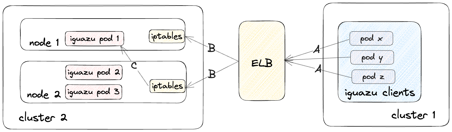
To overcome these challenges, DoorDash has made Kafka a tenant-aware application, which allows different tenants to share the same topic. Figure 1 below provides an overview of the Kafka workflow architecture.
Figure 1: Multi-tenant Kafka Workflow
In this workflow, messages originating from various tenant environments are tagged with distinct tenant information by an agent of OpenTelemetry, or OTEL — an open-source framework that provides tools and software to collect and process telemetry data from cloud-native applications. OTEL uses native Kafka headers to propagate context. Upon receipt by the consumer, the context filter relays messages containing the appropriate tenant information to the processor. This ensures that sandbox consumers mirror the configurations of production consumers and subscribe to the same topic.
To achieve this, we made several changes to Kafka producer and consumer clients as described below.
Kafka producer with context propagation
As explained in a previous post, OTEL provides custom context propagation, which simplifies implementation of multi-tenancy on the Kafka producer side.
Each event sent out by the Kafka producer includes propagated tenant and route information.
Additionally, we have scenarios in which a single service requires multiple sandbox environments. To distinguish which sandbox environment an event is directed toward, we incorporate route information to map a production service application name to a sandbox host. A unique host label is generated upon sandbox deployment. The host label varies between deployments but remains consistent among all pods within the same deployment. The pod machine’s environment variable sets the host label, which provides route information in the context propagation. Both of these contexts can easily be configured through an internal UI tool.
Kafka consumer as a service
In DoorDash, the Asgard framework offers a range of standard libraries that encapsulate commonly used server and client functionalities. Asgard dependencies are presented as a single opaque list, providing all the boilerplate necessary for integrating widely used libraries and hiding their versions behind one Asgard version. Asgard also offers yet-another-markup-language, or YAML, configuration files for various environments such as prod, and sandbox.
Asgard lets product team engineers concentrate solely on implementing the business logic in their services. For Kafka consumers, Asgard runs as a service, only exposing configurations through YAML files while processing the event method for developers.
Figure 2 below shows an overview of Asgard. Thanks to this framework, product team engineers only need to focus on the YAML configuration and Service implementation sections.
Figure 2: Asgard Framework
The Asgard framework allows us to inject multi-tenancy awareness for Kafka consumers in one place, which is then automatically applied to all the product team’s services.
Consumer group isolation
Consumer groups allow Kafka consumers to work together and process events from a topic in parallel. Events sent to the same topic will be load-balanced to all consumers in the same group, meaning the first requirement is to set different consumer groups for various tenants. We offer two ways to do consumer group isolation in a sandbox environment.
The first option is manual configuration, where the user can update the YAML config file and set a different group ID for the sandbox environment.
The second option is auto-generation, which is enabled by default for Asgard Kafka consumers. When running in a sandbox environment, the Asgard Kafka consumer service automatically appends the host label’s suffix to the group ID. This ensures that different sandbox deployments have different consumer groups and that within the same deployment, all consumer pods are part of the same consumer group. This approach ensures proper load balancing of events to all consumers within the same group while maintaining isolation between different tenant groups.
Another important consideration is setting the auto.offset.reset property for the Kafka consumer. In the sandbox environment, we set it to latest by default. This is to prevent the inefficient polling of all existing events in the Kafka cluster whenever a new deployment occurs. Instead, the consumer starts from the latest available event.
Tenant and route context isolation
The test tenant Kafka consumer can now subscribe to the same topic as the production tenant to receive real-time events. The next step is to filter out events not targeted to the current tenant consumers.
To achieve this, we introduced an additional Kafka consumer config field that accepts a list of allowed tenant events. By setting this config field, the Kafka consumer verifies the tenant context information and skips non-matching events. This step ensures that sandbox consumers do not accidentally process events intended for production consumers.
After that, there is another filter based on the route information. We compare the host label retrieved from the environment variable with the one inside the route context header to determine whether the current consumer is the event’s target destination. This step ensures that production and sandbox consumers do not process events that belong to a different tenant. In the absence of the route information, the production tenant processes the doortest events ensuring that test traffic gets processed if there are no sandbox deployed for the service.
For example, our Advertisements Team sought to segregate production and testing events to prevent adverse impacts on our ad serving algorithms caused by production services processing test events. Consequently, they opted for the config pattern, explicitly defining allowedConsumerTenancies for both production and sandbox environments.
In production environment:
kafka: allowedConsumerTenancies: – prod …
In sandbox environment:
kafka: allowedConsumerTenancies: – doortest …
Meanwhile, our Logistics Team preferred not to handle the responsibility of deploying sandboxes solely for processing all test events. They found it safe for their production services to handle both production and test events. However, they aimed to restrict sandboxes to processing specific test events following the deployment of a new release. To achieve this, they simply set enableTenantRouting to true.
kafka: enableTenantRouting: true …
Separately, our Dasher Team wanted to shadow all the production events to test a new alternative architecture. This was safe since the processing of the events did not mutate production data. To achieve this, they simply set enableTenantRouting to false.
kafka: enableTenantRouting: false …
The table in Figure 3 is created by combining tenant and routing context to monitor which Kafka consumer from each environment will handle a specific message.
Consumer Env
Tenant ID (*)
Route Info (*)
Allowed Consumer Tenancies (**)
Process Event?
prod
prod
N/A
prod
Yes
prod
doortest
N/A
prod
No
sandbox
prod
N/A
doortest
No
sandbox
doortest
N/A
doortest
Yes
prod
prod
N/A
both
Yes
prod
doortest
absent
both
Yes
prod
doortest
present
both
No
sandbox
prod
N/A
both
No
sandbox
doortest
sandbox host is not a match
both
No
sandbox
doortest
sandbox host is a match
both
Yes
Figure 3: Kafka message consumption decision table (*) from Kafka event context (**) from yaml config
Putting it all together
With this new multi-tenant aware Kafka, testing Kafka applications in isolation has become easier for the developers. No code changes are required; developers only need to add a single line to the configuration file. This update addresses several use cases, including the consumption of messages with designated tenant IDs and routing contexts. Additionally, it ensures that all Kafka messages are consumed without any being left unprocessed.
This solution ensures that the multi-tenancy paradigm is fully realized in Kafka, providing data isolation between different tenants and avoiding potential issues with data inconsistencies. Overall, this is a crucial step toward achieving a more robust and reliable production environment at DoorDash.
Conclusion
In summary, DoorDash has implemented a multi-tenancy awareness system for both Kafka producers and consumers that makes the production environment’s tech stack more efficient and developer-friendly for testing new features and patches. DoorDash has streamlined the test-and-release process for product team engineers through simple YAML file configurations while ensuring the security and isolation of each tenant’s data. The result is a more robust and simpler testing-in-production environment.
The DoorDash ETA team is committed to providing an accurate and reliable estimated time of arrival (ETA) as a cornerstone DoorDash consumer experience. We want to ensure that every customer can trust our ETAs, ensuring a high-quality experience in which their food arrives on time every time.
With more than 2 billion orders annually, our dynamic engineering challenge is to improve and maintain accuracy at scale while managing a variety of conditions within diverse delivery and merchant scenarios. Here we delve into three critical focus areas aimed at accomplishing this:
Extending our predictive capabilities across a broad spectrum of delivery types and ETA scenarios
Harnessing our extensive data to enhance prediction accuracy
Addressing each delivery’s variability in timing, geography, and conditions
To address these challenges, we’ve developed a NextGen ETA Machine Learning (ML) system, as shown in Figure 1 below. The key novelty in NextGen’s architecture is a two-layer structure which decouples the decision-making layer from the base prediction problem. The goal of the base layer is to provide unbiased accuracy-first prediction with uncertainty estimation through probabilistic predictions. Then the decision layer leverages the base model’s predictions to solve various multi-objective optimization problems for different businesses. This is an evolution from our previous ETA modeling method [1, 2] which focus more on long-tail minimization.
This harnesses state-of-the-art deep learning (DL) algorithms through a novel two-layer ML architecture that provides precise ETA predictions from vast, real-world data sets for optimal robustness and generalizability. The new system introduces:
Multi-task modeling to predict the various types of ETAs via a single model
A probabilistic base layer coupled with a distinct decision layer to quantify and communicate uncertainty
Figure 1. NextGen ETA Machine Learning System
The base layer model outputs a predicted distribution to estimate expected ETA time. The decision layer leverages the base model’s predictions to solve various multi-objective optimization problems for different businesses.
Scaling ETAs Across Different Delivery Types
DoorDash’s ETAs cater to various customer interaction stages and delivery types. Initially, customers can use ETAs on the home page to help them decide between restaurants and other food merchants. The features available for predicting these ETAs are limited because they are calculated before the customer has placed anything in their cart; feature latency must remain low to quickly predict ETAs for all nearby providers.
Delivery types range from a Dasher picking up prepared meals to grocery orders that require in-store shopping, which introduces distinct delivery dynamics.
Historically, this diversity required multiple specialized models, each finely tuned for specific scenarios, leading to a cumbersome array of models. While accurate, this approach proved unsustainable because of the overhead required to adapt and evolve each model separately.
The pivot to multi-task (MT) modeling addresses these challenges head-on. This approach enables us to streamline ETA predictions across different customer touchpoints and delivery types within a singular, adaptable framework.
Nowadays, MT architecture is commonly used in large-scale ML systems such as computer vision and recommendation systems. Our MT architecture consists of a shared heavyweight foundation layer, followed by a specialized lightweight task head for each prediction use case (see “Base Layer” in Figure 1 above).
The consolidated MT model offers four distinct advantages:
We can quickly onboard new ETA prediction use cases by attaching new task heads to the foundation layer and fine-tuning the predictions for the new task.
This model offers a seamless experience across the platform by providing consistent ETA predictions through different stages of the consumer’s journey, including on the home page, store page, and checkout page. Before MT, we trained separate models for each stage, which led to discrepancies in ETA predictions across stages, negatively affecting the consumer experience.
Using the MT model, we can fully leverage the tremendous capacity of DL models, using high-dimensional input features to capture the uncertainty in ETA.
The MT model elegantly solves the data imbalance issue via transfer learning. At DoorDash, certain types of ETA predictions, for example Dasher delivery, are more common than others, such as consumer pick-up. If we train separate models for each use case, the infrequent ones will suffer from lower prediction accuracy. MT improves these infrequent use cases by transferring ETA patterns learned from frequent use cases. For example, MT greatly improved ETA predictions for deliveries in Australia, which previously used a separately trained model.
However, the novel MT architecture involves unique challenges. Model training is more complex because each model must simultaneously learn to predict different ETA use cases. After experimenting with different training strategies, we found that sequentially training different heads, or tasks, achieves the best overall prediction performance. Additionally, there is higher model latency in the MT architecture because of the neural network’s larger number of parameters. We address this through close collaboration with backend engineering teams.
Using Deep Learning to Enhance Accuracy
In our quest to maximize ETA prediction accuracy, we encountered a challenge with our tree-based ML models: they reached a performance plateau beyond which further model enhancements, additional features, or more training data fail to yield significant improvements. Tree-based models also could not generalize effectively to unseen or rare use cases — a common issue with these types of models.
Using tree-based models often resulted in tradeoffs that sacrificed earliness to reduce lateness, and vice versa, rather than improving on-time accuracy. To overcome this and align with our system design goals, we revamped our ETA model architecture from tree-based to neural networks that could provide more accurate, robust, and generalizable ETA prediction performance.
We plan to publish more blog posts on MT ETA model development. Here are high-level summaries of the three key areas we will address:
Feature engineering: We integrated feature-embedding techniques to effectively encapsulate a broad spectrum of high cardinality data. This advancement has significantly refined our model’s ability to discern and learn from intricate patterns unique to specific data segments.
Enhanced model capability: Our model was augmented with advanced components pivotal in detecting both high- and low-level signals and in modeling complex interactions between features.
Flexible optimization: We leveraged the adaptable nature of the DL optimization process to provide flexibility for our model to meet our diverse set of objectives more effectively.
Leveraging Probabilistic Models for More Accurate ETAs
DoorDash believes it is pivotal to ensure customer trust. Customers depend on our delivery time estimates to make choices between restaurants and to organize their schedules. Previously, we used machine learning to produce estimates based on analyzing past delivery data, factoring in various elements like food preparation time and Dasher availability.
However, aspects of the delivery process are inherently uncertain and involve factors we can’t fully predict or control. This unpredictability can affect out accuracy. Consider these scenarios:
Component
Unknown Factor
Potential Impact
Food preparation time
# of sit-down and non-DoorDash restaurant orders
Delay in food readiness
Dasher availability
Whether nearby Dashers will accept the order
Pickup time variability
Parking availability
In dense urban areas, Dashers may have trouble finding parking
Pickup and/or drop-off delays
By factoring in these uncertainties, we aim to refine our delivery estimates, balancing accuracy with the reality of unpredictable factors. We do this by leveraging the innovative two-layer structure which employs aprobabilistic prediction model as the base layer.
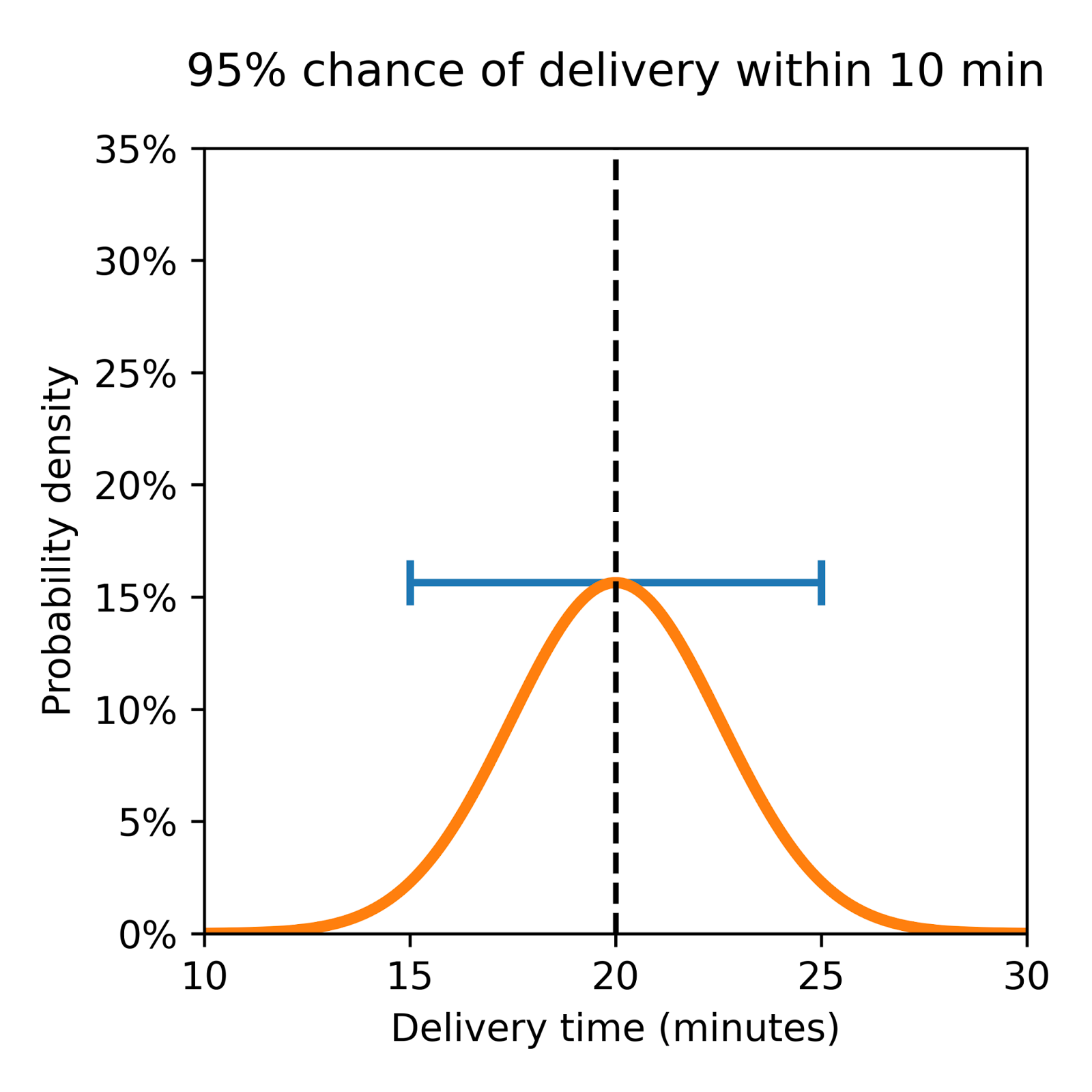
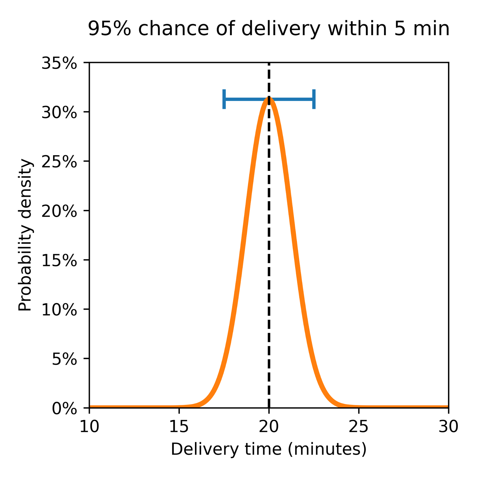
Consider two theoretical deliveries as shown in Figure 2 below, both with a predicted ETA of 20 minutes, but one with a larger variance and a higher chance of being either early or late.
High Uncertainty
Low Uncertainty
This distribution shows a wide spread, indicating significant variability. Although the average ETA is 20 minutes, actual delivery times may vary widely, reflecting a high level of uncertainty.
Here the distribution is closely clustered around the 20-minute mark. This tight grouping suggests that deliveries will likely align closely with the estimated time, indicating lower uncertainty.
Figure 2: Modeling the uncertainty of delivery time via by predicting its probability distribution
These visuals underscore an important concept: It’s as crucial to understand the probability of all possible outcomes via a distribution’s shape and spread as it is to know the mean ETA, or most likely arrival time. That’s why our new base layer was developed to produce a probabilistic forecast of delivery time, giving us a much more developed understanding of uncertainty.
Deep Dive — Evaluating the Accuracy of a Probabilistic Forecast
With our shift to probabilistic forecasts, we encounter a new challenge: Measuring the accuracy of our predictions. Unlike point estimates, where accuracy is assessed in a straightforward manner through metrics like mean absolute error (MAE) or root mean square error (RMSE), probabilistic predictions require a different approach.
Weather forecasting offers valuable insights into what is required to meet this challenge. Forecasters predict probabilities for weather events in a similar manner to our delivery time predictions. In both cases, there’s a single actual outcome, whether it’s a specific temperature or a delivery time, involving two primary metrics: Calibration and accuracy.
Calibration
Probabilistic calibration ensures a model’s predicted distributions align closely with actual outcomes. In other words, realizations should be indistinguishable from random draws from predictive distributions. Consider a weather model that predicts temperature ranges with certain probabilities. A model that consistently underestimates high temperatures likely has a calibration issue.
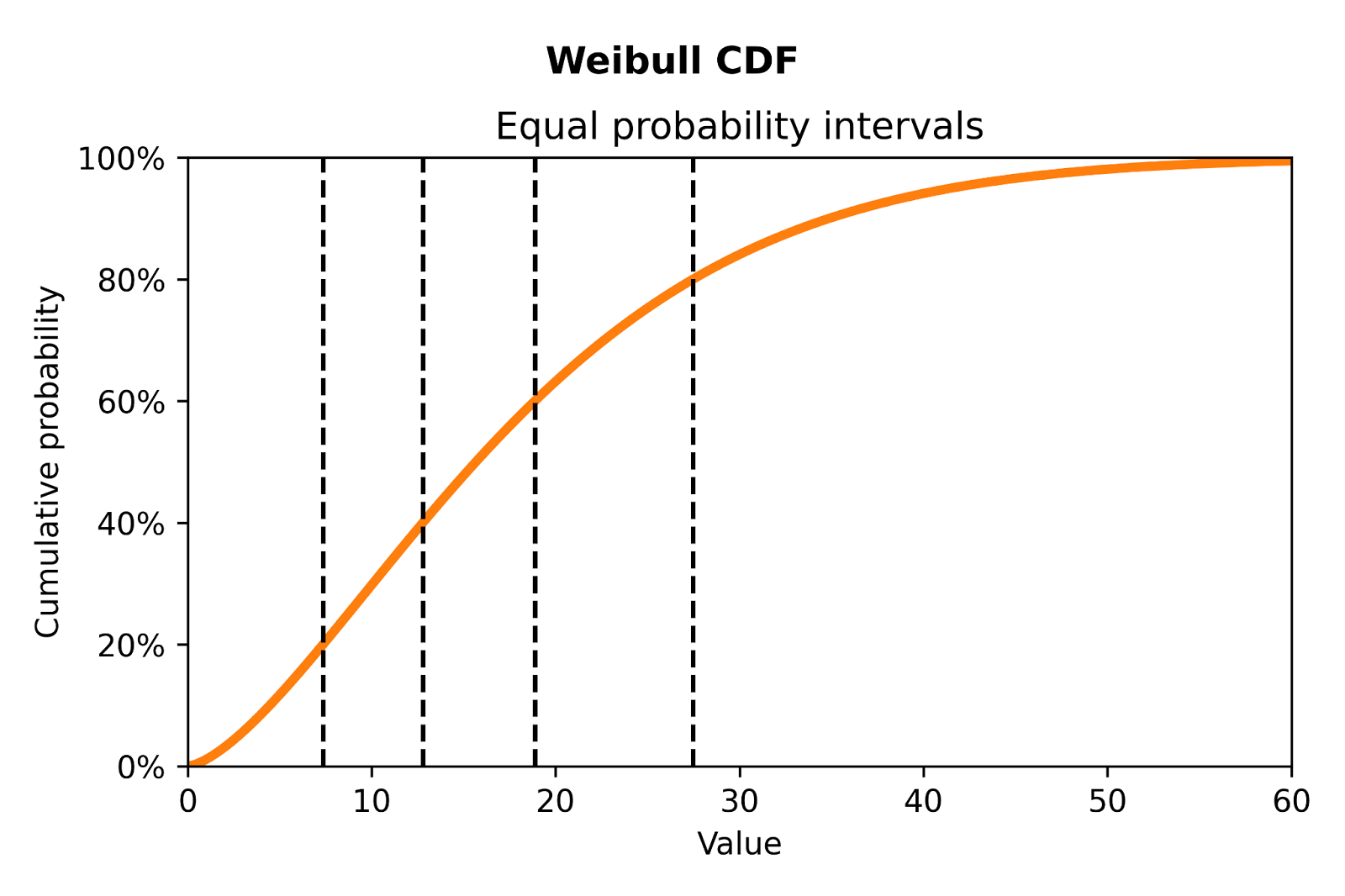
To apply this to DoorDash’s ETA model, imagine our deliveries all have the same underlying distribution. Figure 3 shows lines on a Weibull cumulative distribution function (CDF) that denote five equal probability buckets. If the predicted distribution is accurate, we can expect an equal number of deliveries to land in each bucket.
Figure 3: CDF of Weibull distribution, used to model long-tailed delivery time
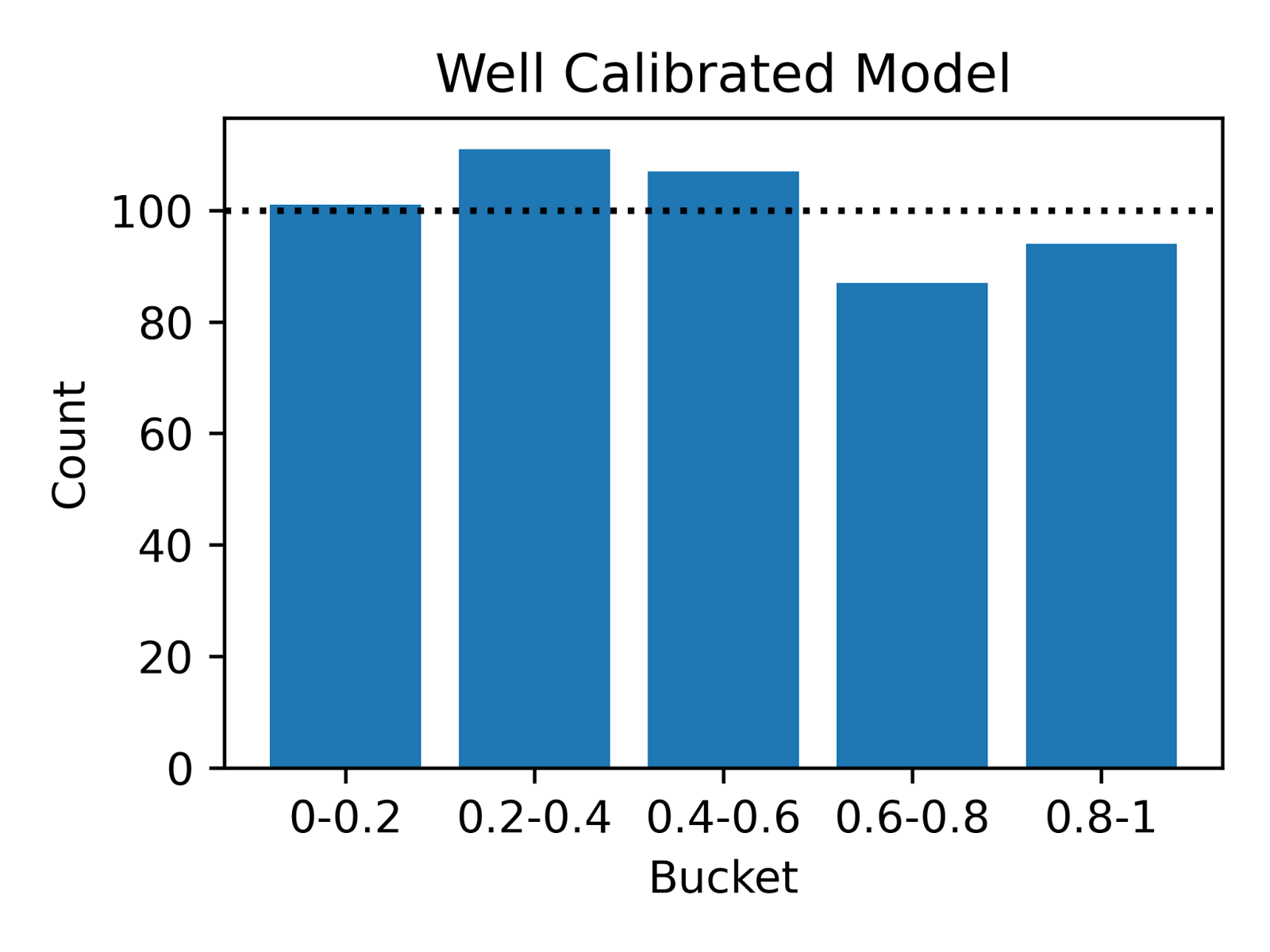
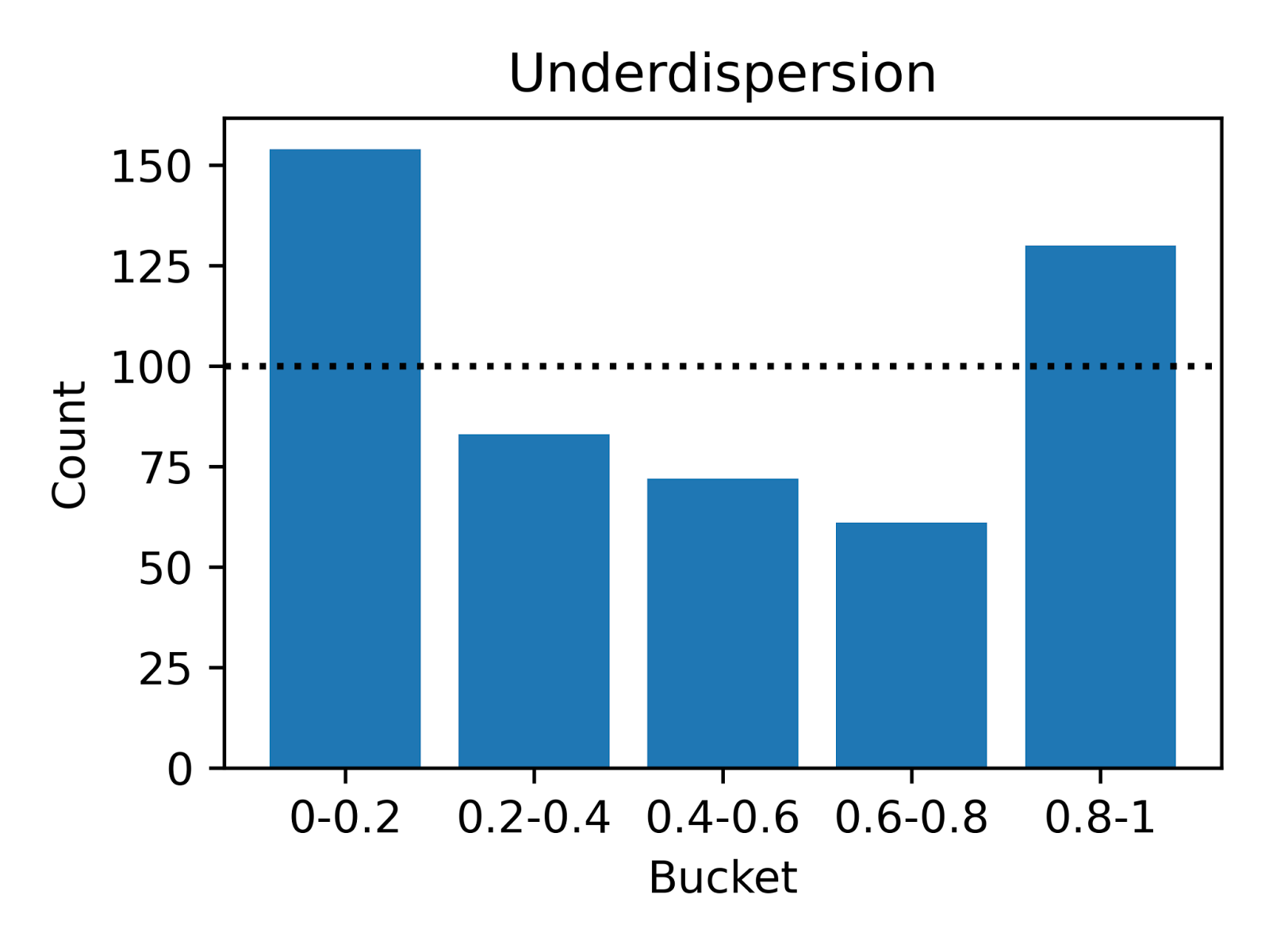
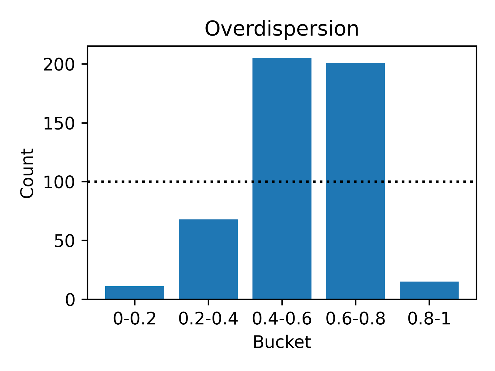
The following simulation illustrates the different types of calibration errors. In Figure 4 below, we show the results of simulating two underlying distributions versus a well-calibrated static predicted distribution. To create a probability integral transform (PIT) histogram visualization, we drew 500 deliveries and plotted the actual delivery times against our predicted quantiles to inspect probabilistic calibration.
Well-Calibrated
Under-Dispersion
Over-Dispersion
Deliveries are evenly distributed across the quantiles, indicating accurate predictions.
A U-shaped pattern suggests the model predicts a wider range than observed, indicating over-caution.
An inverse-U shape reveals the model underestimates variability, missing the extreme cases.
Figure 4: Use PIT to measure the calibration of the predicted probability distribution
These visuals show how well our model captures the real-world variability in delivery times. Calibration is key to ensuring that our predictions are not just accurate for the most likely delivery time, but also reliable and reflective of actual delivery scenarios.
Accuracy
While calibration is essential, it cannot by itself encompass the complete picture of a model’s accuracy. To holistically assess our model, we need a unified metric that can compare different models effectively. Here, we borrow from the weather forecasting field once again, employing a technique known as the continuous ranked probability score (CRPS).
CRPS extends the concept of MAE to probabilistic forecasts. The formula for CRPS is:
CPRS(F(· |X), x) ﹦∫ (F(y|X) – 1{y ≥ x} )2 dy
Where:
F(y|X) represents the CDF of the forecast, conditioned on the covariates X
x is the single observed delivery time for an order
1{y ≥ x} is the indicator function, equal to 1 if y ≥ x and 0 otherwise
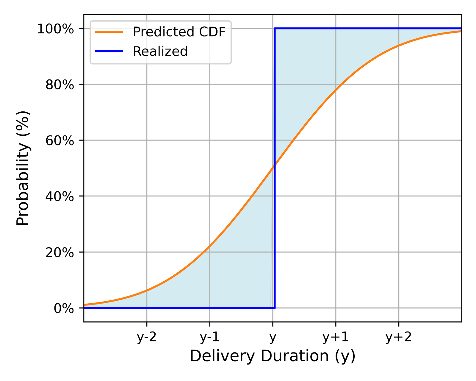
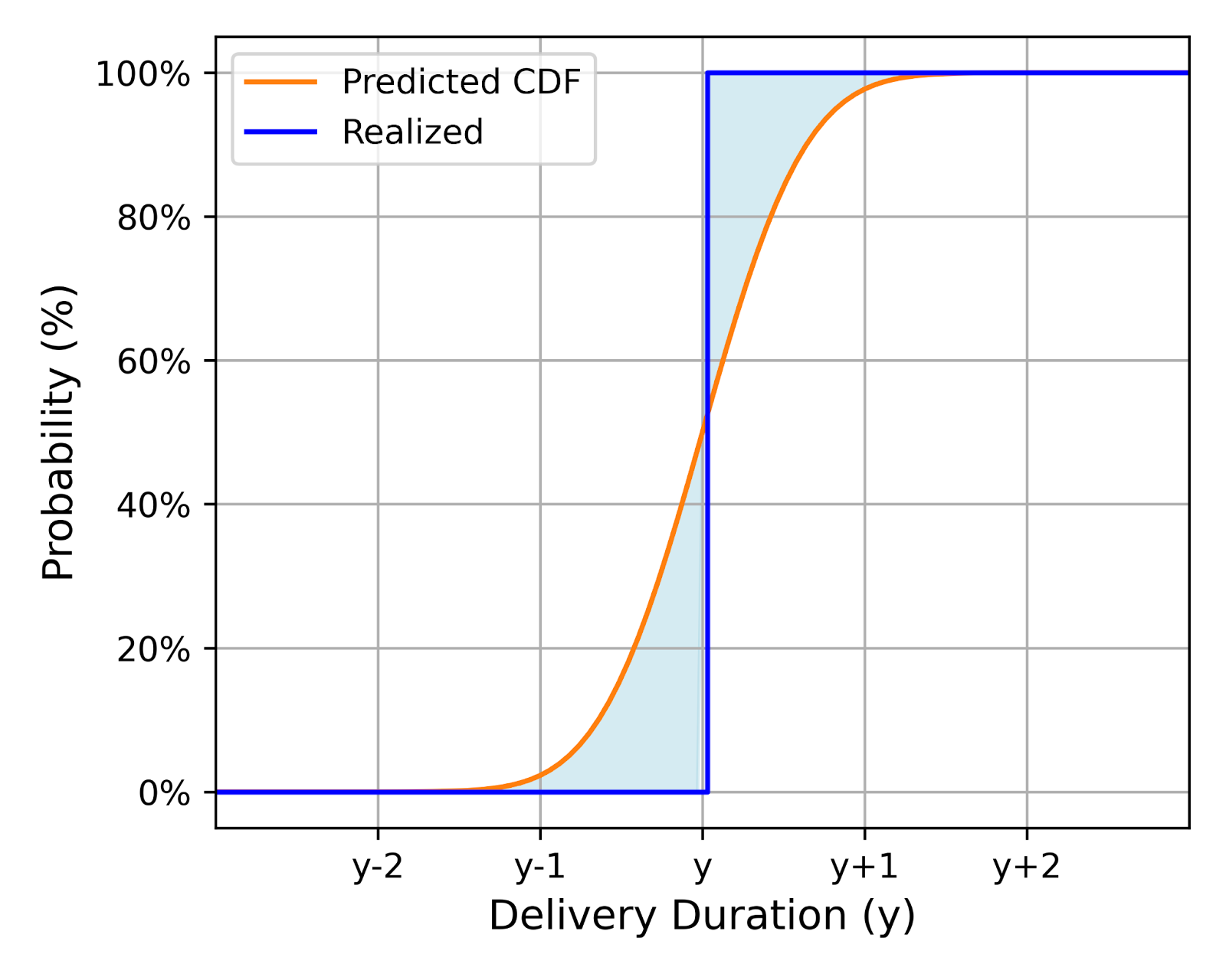
In simpler terms, CRPS measures how well the predicted distribution (every point weighted by its probability) aligns with the actual observed delivery time. Visually, we want to minimize the area between the predicted CDF and a vertical line at the observed delivery time, with a higher CRPS penalty for the area further away from the observed delivery time due to the square. Figure 5 shows two examples of this:
Less Accurate
More Accurate
Shows a larger area between the predicted CDF and the observed time, indicating lower accuracy.
Exhibits a smaller area, suggesting a closer alignment between prediction and reality.
Figure 5: Use CRPS to measure the alignment of predicted distribution with ground truth
By averaging the CRPS across multiple predictions, we derive a single, comparable score for each model. This score is crucial to identify both those areas where our model excels and where it needs refinement, ensuring continuous improvement in ETA predictions. We have made significant strides in the probabilistic prediction and distribution evaluation, marking a milestone in our journey. But this journey is far from over; we anticipate further improvements and breakthroughs as we continue to refine and advance our efforts.
Experiment Results
Combining the above techniques, we developed three versions of NextGen ETA models which all improve consumer outcomes.
Accuracy: Our north star metric for the NextGen ETA metric measures how often a delivery arrives on time according to our prediction and the overall quality of our model
Consistency: Our guardrail metric ensures our ETAs are consistent and that customers don’t see large changes in their ETAs
Figure 6: Accuracy and consistency improvements achieved by next-gen ETA models
Conclusion
At DoorDash, our commitment to providing transparent and accurate information is a fundamental part of fostering trust with our consumers. Understanding that the ETA is crucial for our customers, we’ve dedicated ourselves to enhancing our estimates’ precision. Through embracing advanced predictive modeling with multi-task models, deep learning, and probabilistic forecasts, we’re producing world-class predictions while accounting for real-world uncertainties. This approach doesn’t only improve our service; it reinforces our reputation as a reliable and customer-centric platform, ensuring that every ETA we provide is as accurate and trustworthy as possible.
At DoorDash, we’re committed to fostering a workplace where women have opportunities to develop and drive their careers. As part of our commitment to broadening access to opportunity, we recognize the importance of celebrating the past as we continue to invest in growing women into future leaders at DoorDash.
This March, in partnership with our Women@ Employee Resource Group, we’re celebrating Women’s History Month through the 2024 theme of “Women who advocate for Equity, Diversity, and Inclusion.” To celebrate, we’re hosting a series of in-person and virtual events throughout the month.
We’ll kick off our slate of inclusive events with a fireside chat with DoorDash’s Customer Support & Integrity team, featuring panelists:
Arielle Salomon, VP of Customer Experience & Integrity
Erica Parker, Director, People Business Partners
Jessica Morse, Director of Trust & Safety
Melissa Smith, OE Senior Manager, CXI
Aubrey Reynolds, Senior Manager, Marketplace Live Operations
Madison Oeff, Strategy & Operations Manager, T&S
Melissa Forziat will lead a goal setting webinar and author, women’s empowerment coach, and international speaker Ifeoma Esonwune will join us for a special session on self-advocacy.
Through four #IAmRemarkable sessions, our people are invited to celebrate their achievements in the workplace and beyond as they learn the importance of self promotion. And we’ll wrap the month with a series of virtual Fidelity sessions, where individuals will learn about financial equity and inclusion, ensuring equal access to financial services.
All month long, we’re encouraging our people to celebrate women at DoorDash who have played an instrumental role in supporting their peers while making room at the table through thank-you notes and virtual words of encouragement.
We will continue to prioritize investing in and creating opportunities for historically underrepresented people. Our success as a company is firmly rooted in our inclusive culture and in advancing diversity throughout DoorDash to ensure we reflect the global audiences we serve. We are proud to offer learning and development opportunities year-round to corporate team members that highlight opportunities for our allies and the community.
We reviewed the architecture of our global search at DoorDash in early 2022 and concluded that our rapid growth meant within three years we wouldn’t be able to scale the system efficiently, particularly as global search shifted from store-only to a hybrid item-and-store search experience.
Our analysis identified Elasticsearch as our architecture’s primary bottleneck. Two primary aspects of that search engine were causing the trouble: its document-replication mechanism and its lack of support for complex document relationships. In addition, Elasticsearch does not provide internal capabilities for query understanding and ranking.
We decided the best way to address these challenges was to move away from Elasticsearch to a homegrown search engine. We chose Apache Lucene as the core of the new search engine. The Search Engine uses a segment-replication model and separates indexing and searching traffic. We designed the index to store multiple types of documents with relations between them. Following the migration to DoorDash’s Search Engine, we saw a 50% p99.9 latency reduction and a 75% hardware cost decrease.
Path to Our Search Engine
We wanted to design the new system as a horizontally scalable general-purpose search engine capable of scaling to all traffic – indexing or searching – by adding more replicas. We also designed the service to be a one-stop solution for all DoorDash teams that need a search engine.
Apache Lucene, the new system’s foundation, provides a mature information retrieval library used in several other systems, including Elasticsearch and Apache Solr. Because the library provides all the necessary primitives to create a search engine, we only needed to design and build opinionated services to run on top of the library.
The Search Engine Components
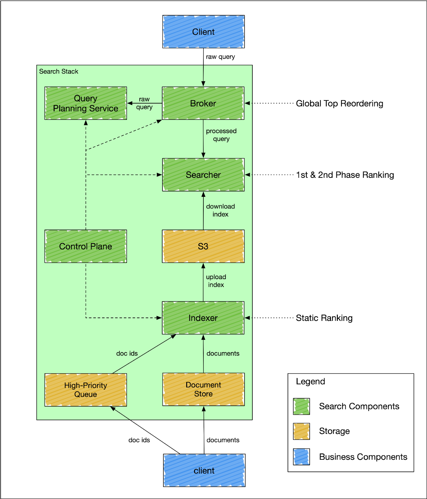
To address scalability challenges, we adopted a segment-replication model. We split indexing and searching responsibilities into two distinct services – indexer and searcher, as shown in Figure 1 below. The indexer is a non-replicated service that handles all incoming indexing traffic and uploads newly created index segments to S3 for searcher consumption. The searcher is a replicated service that serves queries against the index downloaded from S3.
Because the searcher is not responsible for indexing traffic, it only needs to scale proportionally to the search traffic. In other words, the searcher will not be affected by any volume of indexing traffic. The indexer is not a replicated service; horizontally scaling the indexer means increasing the number of index shards, which could be expensive. To alleviate that issue, we split the indexing traffic into bulk and high-priority updates. The high-priority updates are applied immediately, while the bulk updates are only applied during the next full index build cycle, usually every six hours.
Figure 1: The Search Stack Architecture
It’s insufficient to query an index with only indexers and searchers because the index could consist of multiple index shards. Therefore, we designed the broker service as an aggregation layer that fans out the query to each relevant index shard and merges the results. The broker service also rewrites the user’s raw query using a query understanding and planning service.
We also needed a component that could do query understanding and query planning. The component needs to know the specifics of a particular index and the business domain where the index is used. It would be suboptimal to outsource this responsibility to the client because each client would need to replicate this logic and keep updated. But if the logic were consolidated into the query planning service, the clients would only need to know the high-level interface without getting into all the details about query internals.
General Purpose Search Engine
As a general-purpose search engine, the Search Engine must power not only DoorDash’s store and item search but also must be available for every team that needs an information retrieval solution. That meant designing the system to provide a clear separation between core search and business logic. A user must be able to express business logic with little to no code changes and that logic must be completely isolated from the logic of other users.
The best approach to separating core search and business logic would be to introduce a declarative configuration for index schema and provide a generic query language. The index schema allows users to define strongly typed documents, or namespaces, and create relationships between the namespaces. A namespace definition consists of three primary parts:
Indexed fields are fields the indexer processes and writes (or not) in some shape or form into the inverted index. The Search Engine supports all Apache Lucene fields, including text, numeric doc values, dimensional points, and KNN vectors.
Computed fields are fields computed dynamically during query time based on inputs such as the query, the indexed fields, and other computed fields. The computed fields framework provides a means to express complex ranking functions and custom business logic; as an example, we can define a BM25 or an ML model as a computed field.
Query planning pipelines define the logic of how to process raw client queries into the final form used to retrieve and rank documents. The primary objective is to encapsulate the business logic and store it in one place. For example, a client calling DoorDash’s global search does not need all the complexity of the geo constraints if the logic is implemented in a query planning pipeline. The client would only need to supply the search with coordinates or a geo-hash of the delivery address and the name of the query planning pipeline to invoke.
In addition to the flexible index schema model, we created an SQL-like API as a powerful and flexible search query to allow customers to express their business logic with minimal code changes. The API provides a set of standards for search engine operators, such as keyword groups, filter constraints, sorting by fields, and a list of returned fields. Additionally, the Search Engine supports join and dedupe operators.
To support the join operator, we designed relationships between namespaces. A relationship can be either local-join or block-join. The local-join relationship is set between parent and child namespaces to guarantee that a child document will be added to the index shard only if a parent document references it. The nested relationship works similarly to the local-join relationship, but the parent and the children must be indexed together as a single block. Both options have advantages and weaknesses. The local-join relationship allows updating documents independently but requires executing queries sequentially. The nested relationship allows faster query execution but requires reindexing the whole document block.
Tenant Isolation and Search Stacks
Data and traffic isolation are important for users of a general-purpose search engine. To provide this isolation, we designed a search stack — a collection of search services dedicated to one particular index. A component of one search stack only knows how to build or query it’s index. Thus, sudden issues in one search stack will not cause any issues for other search stacks. Additionally, we can easily account for all resources provisioned by tenants to keep them accountable.
Search stacks are great for isolating tenants’ index schemas and services. Additionally, we wanted to find an easy way to mutate index schema and stack configuration without worrying about backward compatibility of changes. Users must be able to make changes in the index schema or fleet configuration and deploy them as soon as the changes do not have internal contradictions.
We designed a special component called a control plane — an orchestration service that is responsible for stack mutation, as shown in Figure 2 below. The control plane deploys stacks by gradually deploying a new generation and descaling the previous one. A generation has a fixed version of the search Docker image to deploy. All search components in the same generation have the same code version, index schema, and fleet configuration. The components inside a generation are isolated and can only communicate with other components within the same generation. A searcher can only consume an index produced by the indexer of the same generation, and a broker can only query searchers of the same generation.
Figure 2: Deployment of a New Stack Generation
This simplifies user-side changes in exchange for a more complex deployment pipeline. The control plane deploys a new generation of a stack every six hours, although that can be changed to any arbitrary timing. It starts by cutting a new release of the search repository. When the release is ready, the control plane deploys a new stack, starting from the indexer. The indexer builds a new index from scratch — full index build — and catches up with high-priority updates. After the indexer signals the new index is ready, the control plane starts gradually scaling the serving side of the current generation and descaling the previous one.
Conclusion
We spent 2023 implementing the Search Engine and migrating DoorDash to it. In the first half of the year, we delivered the initial version of the system and migrated the global store search. That led to a two-fold reduction of the store retrieval latency and a four-fold reduction of the fleet cost.
During the second half of the year, we added support for the join queries, query planning, and support for ML-ranking functions. We migrated the query understanding from the client to the query planning layer. Now, any client can call the search without replicating complex query-building logic. The join query and ML ranking are used to do global item searches without first calling the store index. These features contributed to significant improvements in the precision and recall of the item index.
Migrating to an in-house search engine has given us tight control over the index structure and the query flow. The Search Engine lets us create a flexible, generic solution with features optimized for specific DoorDash needs and the scalability to grow at the same pace as DoorDash’s business.
Business Policy Experiments Using Fractional Factorial Designs
At DoorDash, we constantly strive to improve our experimentation processes by addressing four key dimensions, including velocity to increase how many experiments we can conduct, toil to minimize our launch and analysis efforts, rigor to ensure a sound experimental design and robustly efficient analyses, and efficiency to reduce costs associated with our experimentation efforts.
Here we introduce a new framework that has demonstrated significant improvements in the first two of these dimensions: velocity and toil. Because DoorDash conducts thousands of experiments annually that contribute billions in gross merchandise value, it is critical to our business success that we quickly and accurately test the maximum number of hypotheses possible.
We have found that even as we enhance experimental throughput, we can also streamline the associated setup effort. In certain domains, such as campaign management in CRM, it can be time-consuming to designate and apply business policies to different user segments. The effort tends to be linearly correlated with the number of policies to be tested; additionally, the process can be prone to errors because of the need to conduct multiple manual steps across various platforms.
Our proposed framework, as outlined in this paper, increased experimental velocity by 267% while reducing our setup efforts by 67%. We found that the benefits generally are more pronounced when a model includes multiple factors, such as a feature or attribute of a policy, and levels, such as the value of a factor.
In addition to increasing velocity and reducing toil, our framework also provides a mechanism for testing the assumptions underlying an experiment’s design, ensuring a consistently high level of rigor.
A/B testing for CRM campaign optimization
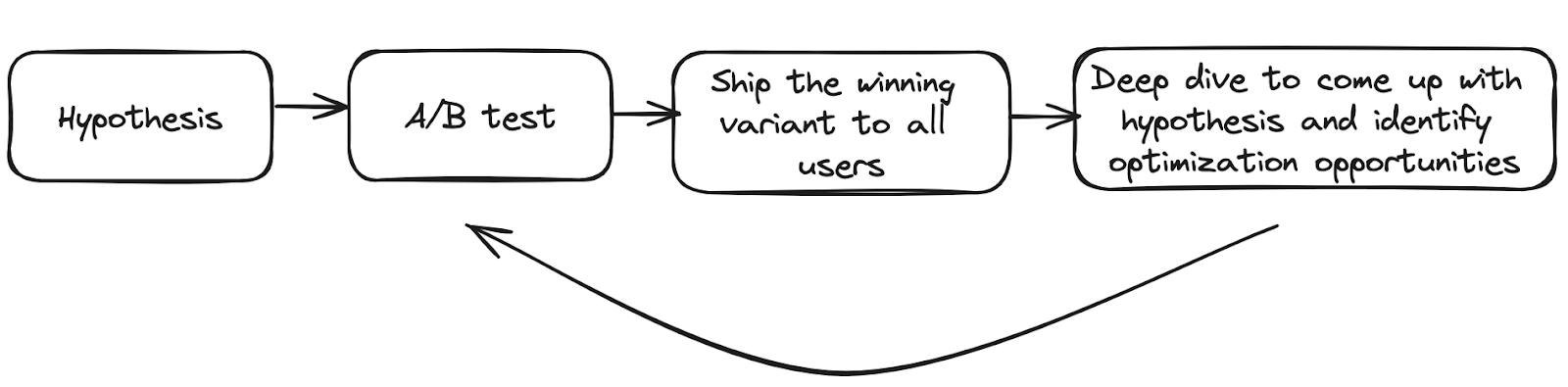
The consumer retention marketing team aims to build a lasting relationship with customers from the first moment they engage with DoorDash by presenting relevant marketing content to drive them to return. Like many businesses, we often use A/B tests to continually iterate on our best policy, choosing from the huge number of options in our policy space. Figure 1 below shows our typical experimentation lifecycle:
Figure 1: Experimentation lifecycle in CRM
A number of challenges dampen our speed and increase the effort required to conduct experiments, including:
High implementation costs: Unlike conventional web experiments, if we were to A/B test several policies at once, the setup implementation costs for randomized user segments could be extremely high.
Budget constraints: Our limited marketing budget constraints our testing capabilities. Because each policy requires a minimum sample size to detect an effect, we can only assess a limited number of policies.
Long-term metrics: Many metrics crucial to our evaluation, such as retention, require an extended measurement period, slowing our velocity.
Sequential testing risks: Testing policies sequentially over time exposes experiments to potential risks, including shifts in business priorities. This may hamper implementation of optimal features while interfering with future iterations because of additional factors such as budget constraints and resource reallocation.
Because of these challenges and other issues, we can only test and compare a limited number of policies each quarter.
Another challenge worth mentioning is personalization, which we believe is key to making our marketing campaigns relevant and driving better long-term engagement. In a perfect world, we would test all possible policies and run a heterogeneous treatment effect, or HTE, model to identify the best policy for each consumer’s historical data. However, because we have only training data with limited policies/campaigns and a small sample size, we are prevented from making the most of an HTE model.
Stay Informed with Weekly Updates
Subscribe to our Engineering blog to get regular updates on all the coolest projects our team is working on
Please enter a valid email address.
Thank you for Subscribing!
Applying fractional factorial design to the business policies space
In light of the challenges of prolonged experiment duration, high setup costs, and difficulty in identifying personalized policies, we created a framework that uses fractional factorial design to solve the problem. The following is a brief overview of the framework’s intuition; readers seeking detailed insights are encouraged to explore our full paper on Arxiv.
Step 1) Factorization — break down the hypothesis into factors
Promotion policies traditionally have been treated at the experimentation phase as monolithic units and not as combinations of distinct components. Our framework’s first innovation is to break down the campaign policy space into factors to create a foundation for the factorial design framework. In our project, we broke down the policy space into four distinct building blocks: promo spread, discount, triggering timing, and messaging, as shown in Figure 2.
After creating these four building blocks — one with three levels and the others with two — we have 24 combinations. Recall the setup effort referenced above; there are major operational challenges in setting up such a 24-arm marketing campaign in one shot. To solve this problem, we make assumptions on higher-order interactions, for example no interaction effects. Don’t worry; we will test these assumptions later. We then apply fractional factorial design to shrink the number of variants from 24 to eight, which reduces the setup cost by 66%. The different methodologies to conduct fractional factorial design are detailed in the full paper.
Figure 3: In-sample and out-of-sample variants [1]
Step 3) Launch the experiment by including an additional out-of-sample variant
After we select eight in-sample variants to launch, we intentionally select a ninth variant which we will launch at the same time. We include an out-of-sample variant so that we can end-to-end test our assumptions about interaction effects. It is critical to validate with data any assumptions made based on our business intuition.
Step 4) Collect the data and validate the model assumption
After the experiment is launched and it reaches the predetermined sample size, we use the collected data to validate the model. On a high level, we use the data from the in-sample variants to predict the metric in the ninth validation variant. If the model is correct, the prediction should be close to the observed value. We discuss how to validate in greater detail in our paper.
Step 5) Estimate the treatment effect for each factor and policy
After the data is collected and the model assumption is validated through the out-of-sample variant, we estimate the treatment effect for each factor level and interaction if included in the model. We then can derive the treatment effect for all possible promo policy permutations.
Step 6) Use an ML model to estimate heterogeneous treatment effect
After the analysis of the average treatment effect, we consider personalized campaigns. The joint test we describe in our paper helps determine whether personalization is needed and what user characteristics are useful for personalization. If personalization buys us incremental value, we can apply a machine learning model to learn the heterogeneous treatment effect. In our paper, we discuss two general categories of models and a way to adjust the bias. In our example, the HTE model can generate 2% more profit than a single optimal campaign for all users.
Broader Applications
By breaking down policies into factors, we can leverage the factorial design to test more hypotheses simultaneously. By making assumptions about the interaction effects, we can reduce the number of in-sample variants that must be implemented.
In our specific business context, the framework improved on current methods by helping us discover the personalized policy with a 5% incremental profit while delivering 267% faster experimentation and 67% lower setup costs.
We believe the framework can be applied more generally to other domain areas where experiments are slowed by limited sample size and/or where setup or configuration costs increase with the number of variants or arms being tested. In our next steps, we plan to apply the framework to other domain areas at DoorDash and also further improve and productionize the personalized HTE model. For those seeking a deeper understanding, we encourage readers to delve into our preprint on Arxiv.
Acknowledgements
We would like to thank our retention marketing partners, Kristin Mendez, Meghan Bender, Will Stone, and Taryn Riemer, for helping us set up and launch the experiments throughout this research; we would also like to acknowledge the contributions of the data science and experimentation team colleagues, especially Qiyun Pan, Caixia Huang, and Zhe Mai. Finally, we want to thank our leadership Gunnard Johnson, Jason Zheng, Sudhir Tonse and Bhawana Goel for sponsoring this research and providing us with guidance along the way.
Black History Month holds profound significance as it is a dedicated time to honor and acknowledge Black individuals’ invaluable contributions, achievements, and struggles throughout history. As we make progress toward creating a workplace that engages people of all backgrounds while fostering an environment of diversity, equity, and inclusion, Black History Month provides an opportunity for month-long observance and a deeper understanding of the resilience, courage, and brilliance of Black leaders, activists, artists, inventors, and countless unsung heroes who have shaped history despite enduring systemic injustices.
This February, in collaboration with our Black@ Employee Resource Group, we continue to acknowledge and reflect on the significance of Black history while embracing and embodying this year’s theme of African Americans & the Arts.
Beginning on February 1 and throughout the month, we’re hosting a series of in-person and virtual events. We’ll kick off the month with a Virtual Black Art Tour, hearing immersive stories from an expert art and culture guide. Later in the month, we’ll have Black History Month-themed trivia followed by an afternoon of short films centering on Blackness and Black Creators, and later we’ll be joined by artist Mikael Owunna to chat about the art of pride and self-love.
Our Black@ ERG members will take part in a Lunch ‘N’ Learn series to inspire and learn from each other and we’ll celebrate the month during a Black@ members meeting. In our New York and Tempe office spaces, we’ll learn the art of movement through a hosted in-office yoga class guided by an onsite instructor.
To close our Black History Month, we’ll host our first-ever Black@ Dashmart initiative, where we are honored and excited to highlight and celebrate some of the many Black leaders we have in our DashMarts, and give them a new forum to tell the stories of their careers and development.
To continue our work in engaging black-owned businesses, our Workplace Services and DashMart teams are partnering to highlight black-owned snack products as part of our corporate office snack program during Black History Month, which includes Rude Boy Cookies, Elise Dessert Company, Maya’s Bakes, Mirellis Ice Cream, Staten Sweets, and more.
We will continue to prioritize investing in and advancing opportunities for historically underrepresented people. Our success as a company is firmly rooted in our inclusive culture and in advancing diversity throughout DoorDash to ensure we reflect the global audiences we serve, with learning and development opportunities available to corporate team members covering topics such as how to support allyship and anti-racism, dealing with microaggression, being an inclusive organization, and more.
In the realm of distributed databases, Apache Cassandra stands out as a significant player. It offers a blend of robust scalability and high availability without compromising on performance. However, Cassandra also is notorious for being hard to tune for performance and for the pitfalls that can arise during that process. The system’s expansive flexibility, while a key strength, also means that effectively harnessing its full capabilities often involves navigating a complex maze of configurations and performance trade-offs. If not carefully managed, this complexity can sometimes lead to unexpected behaviors or suboptimal performance.
In this blog post, we walk through DoorDash’s Cassandra optimization journey. I will share what we learned as we made our fleet much more performant and cost-effective. Through analyzing our use cases, we hope to share universal lessons that you might find useful. Before we dive into those details, let’s briefly talk about the basics of Cassandra and its pros and cons as a distributed NoSQL database.
What is Apache Cassandra?
Apache Cassandra is an open-source, distributed NoSQL database management system designed to handle large amounts of data across a wide range of commodity servers. It provides high availability with no single point of failure. Heavily inspired by Amazon’s 2007 DynamoDB, Facebook developed Cassandra to power its inbox search feature and later open-sourced it. Since then, it has become one of the preferred distributed key-value stores.
Cassandra pros
Scalability: One of Cassandra’s most compelling features is its exceptional scalability. It excels in both horizontal and vertical scaling, allowing it to manage large volumes of data effortlessly.
Fault tolerance: Cassandra offers excellent fault tolerance through its distributed architecture. Data is replicated across multiple nodes, ensuring no single point of failure.
High availability: With its replication strategy and decentralized nature, Cassandra guarantees high availability, making it a reliable choice for critical applications.
Flexibility: Cassandra supports a flexible schema design, which is a boon for applications with evolving data structures.
Write efficiency: Cassandra is optimized for high write throughput, handling large volumes of writes without a hitch.
Cassandra cons
Read performance: While Cassandra excels in write efficiency, its read performance can be less impressive, especially in scenarios involving large data sets with frequent reads at high consistency constraints.
Expensive to modify data: Because Cassandra is a log structured merge tree where the data written is immutable, deletion and updates are expensive. Especially for deletes, it can generate tombstones that impact performance. If your workload is delete- and update-heavy, a Cassandra-only architecture might not be the best choice.
Complexity in tuning: Tuning Cassandra for optimal performance requires a deep understanding of its internal mechanisms, which can be complex and time-consuming.
Consistency trade-off: In accordance with the CAP theorem, Cassandra often trades off consistency for availability and partition tolerance, which might not suit all use cases.
Cassandra’s nuances
The nuances surrounding Cassandra’s application become evident when weighing its benefits against specific use case requirements. While its scalability and reliability are unparalleled for write-intensive applications, one must consider the nature of their project’s data and access patterns. For example, if your application requires complex query capabilities, systems like MongoDB might be more suitable. Alternatively, if strong consistency is a critical requirement, CockroachDB could be a better fit.
In our journey at DoorDash, we navigated these gray areas by carefully evaluating our needs and aligning them with Cassandra’s capabilities. We recognized that, while no system is a one-size-fits-all solution, with meticulous tuning and understanding Cassandra’s potential could be maximized to meet and even exceed our expectations. The following sections delve into how we approached tuning Cassandra — mitigating its cons while leveraging its pros — to tailor it effectively for our data-intensive use cases.
Stay Informed with Weekly Updates
Subscribe to our Engineering blog to get regular updates on all the coolest projects our team is working on
Please enter a valid email address.
Thank you for Subscribing!
Dare to improve
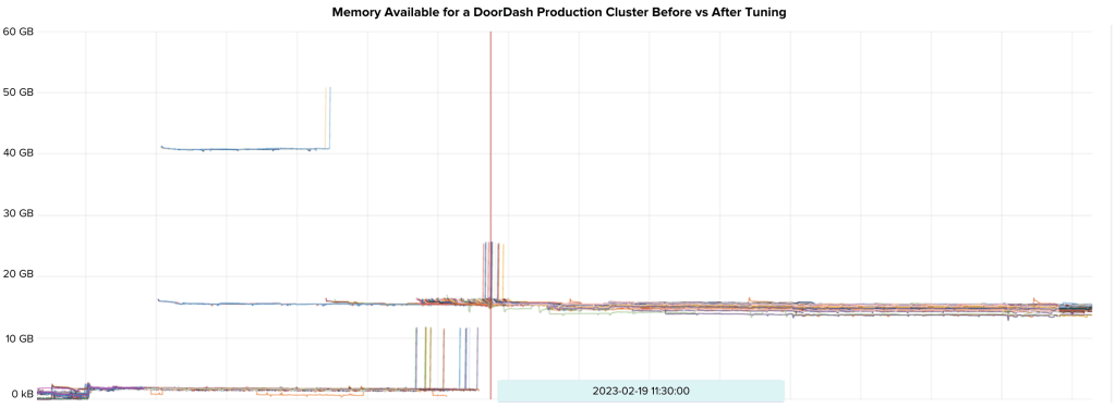
Because of DoorDash’s fast growth, our usage of Cassandra has expanded rapidly. Despite enhancing our development speed, this swift growth left a trail of missed opportunities to fine-tune Cassandra’s performance. In an attempt to seize some of those opportunities, the Infrastructure Storage team worked closely with product teams on a months-long tuning effort. The project has delivered some amazing results, including:
~35% in cost reduction for the entire Cassandra fleet
For each $1 we spend, we are able to process 59 KB of data per second vs. 23 KB, a whopping 154% unit economics improvement
Figure 1: Total number of nodes in Cassandra fleet
In the following section, we will explore specific examples from our fleet that may be applicable to other use cases.
Design your schema wisely from the beginning
The foundational step to ensuring an optimized Cassandra cluster is to have a well-designed schema. The design choices made at the schema level have far-reaching implications for performance, scalability, and maintainability. A poorly designed schema in Cassandra can lead to issues such as inefficient queries, hotspots in the data distribution, and difficulties in scaling. Here are some key considerations for designing an effective Cassandra schema:
Understand data access patterns: Before designing your schema, it’s crucial to have a clear understanding of your application’s data access patterns. Cassandra is optimized for fast writes and efficient reads, but only if the data model aligns with how the data will be accessed. Design your tables around your queries, not the other way around.
Effective use of primary keys:The primary key in Cassandra is composed of partition keys and clustering columns. The partition key determines the distribution of data across the cluster, so it’s essential to choose a partition key that ensures even data distribution while supporting your primary access patterns. Clustering columns determine the sort order within a partition and can be used to support efficient range queries.
Avoid large partitions: Extremely large partitions can be detrimental to Cassandra’s performance. They can lead to issues like long garbage collection pauses, increased read latencies, and challenges in compaction. Design your schema to avoid hotspots and ensure a more uniform distribution of data.
Normalization vs. denormalization: Unlike traditional relational database management systems, or RDBMS, Cassandra does not excel at joining tables. As a result, denormalization is often necessary. However, it’s a balance; while denormalization can simplify queries and improve performance, it can also lead to data redundancy and larger storage requirements. Consider your use case carefully when deciding how much to denormalize.
Consider the implications of secondary indexes: Secondary indexes in Cassandra can be useful but come with trade-offs. They can add overhead and may not always be efficient, especially if the indexed columns have high cardinality or if the query patterns do not leverage the strengths of secondary indexes.
TTL and tombstones management: Time-to-live, or TTL, is a powerful feature in Cassandra for managing data expiration. However, it’s important to understand how TTL and the resulting tombstones affect performance. Improper handling of tombstones can lead to performance degradation over time. If possible, avoid deletes.
Update strategies: Understand how updates work in Cassandra. Because updates are essentially write operations, they can lead to the creation of multiple versions of a row that need to be resolved at read time, which impacts performance. Design your update patterns to minimize such impacts. If possible, avoid updates.
Choose your consistency level wisely
Cassandra’s ability to configure consistency levels for read and write operations offers a powerful tool to balance between data accuracy and performance. However, as with any powerful feature, it comes with a caveat: Responsibility. The chosen consistency level can significantly impact the performance, availability, and fault tolerance of your Cassandra cluster, including the following areas:
Understanding consistency levels: In Cassandra, consistency levels range from ONE (where the operation requires confirmation from a single node) to ALL (where the operation needs acknowledgment from all replicas in the cluster). There are also levels like QUORUM (requiring a majority of the nodes) and LOCAL_QUORUM (a majority within the local data center). Each of these levels has its own implications on performance and data accuracy. You can learn more about those levels in the configurations here.
Performance vs. accuracy trade-off:Lower consistency levels like ONE can offer higher performance because they require fewer nodes to respond. However, they also carry a higher risk of data inconsistency. Higher levels like ALL ensure strong consistency but can significantly impact performance and availability, especially in a multi-datacenter setup.
Impact on availability and fault tolerance: Higher consistency levels can also impact the availability of your application. For example, if you use a consistency level of ALL, and even one replica is down, the operation will fail. Therefore, it’s important to balance the need for consistency with the potential for node failures and network issues.
Dynamic adjustment based on use case:One strategy is to dynamically adjust consistency levels based on the criticality of the operation or the current state of the cluster. This approach requires a more sophisticated application logic but can optimize both performance and data accuracy.
Tune your compaction strategy (and bloom filter)
Compaction is a maintenance process in Cassandra that merges multiple SSTables, or sorted string tables, into a single one. Compaction is performed to reclaim space, improve read performance, clean up tombstones, and optimize disk I/O.
Users should choose from three main strategies to trigger compaction in Cassandra users based on their use cases. Each strategy is optimized for different things:
Size-tiered compaction strategy, or STCS
Trigger mechanism:
The strategy monitors the size of SSTables. When a certain number reach roughly the same size, the compaction process is triggered for those SSTables. For example, if the system has a threshold set for four, when four SSTables reach a similar size they will be merged into one during the compaction process.
When to use:
Write-intensive workloads
Consistent SSTable sizes
Pros:
Reduced write amplification
Good writing performance
Cons:
Potential drop in read performance because of increased SSTable scans
Merges older and newer data over time
You must leave much larger spare disk to effectively run this compaction strategy
Leveled compaction strategy, or LCS
Trigger mechanism:
Data is organized into levels. Level 0 (L0) is special and contains newly flushed or compacted SSTables. When the number of SSTables in L0 surpasses a specific threshold (for example 10 SSTables), these SSTables are compacted with the SSTables in Level 1 (L1). When L1 grows beyond its size limit, it gets compacted with L2, and so on.
When to use:
Read-intensive workloads
Needing consistent read performance
Disk space management is vital
Pros:
Predictable read performance because of fewer SSTables
Efficient disk space utilization
Cons:
Increased write amplification
TimeWindow compaction strategy, or TWCS
Trigger mechanism:
SSTables are grouped based on the data’s timestamp, creating distinct time windows such as daily or hourly. When a time window expires — meaning we’ve moved to the next window — the SSTables within that expired window become candidates for compaction. Only SSTables within the same window are compacted together, ensuring temporal data locality.
When to use:
Time-series data or predictable lifecycle data
TTL-based expirations
Pros:
Efficient time-series data handling
Reduced read amplification for time-stamped queries
Immutable older SSTables
Cons:
Not suitable for non-temporal workloads
Potential space issues if data within a time window is vast and varies significantly between windows
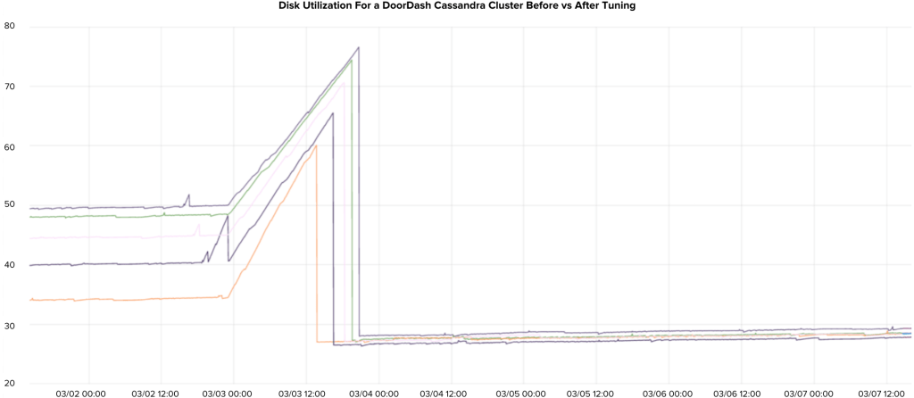
In our experience, unless you are strictly storing time series data with predefined TTL, LCS should be your default choice. Even when your application is write-intensive, the extra disk space required by progressively large SSTables under STCS makes this strategy unappealing. LCS is a no-brainer in read-intensive use cases. Figure 2 below shows the amount of disk usage drop after switching compaction strategy and cleanups.
Figure 2: Disk utilization drop after compaction strategy tuning
It’s easy to forget that each compaction strategy should have a different bloom filter cache size. When you switch between compaction strategies, do not forget to adjust this cache size accordingly.
STCS default bloom filter setting: The default setting for STCS usually aims for a balance between memory usage and read performance. Because STCS can lead to larger SSTables, the bloom filter might be configured as slightly larger than what would be used in LCS to reduce the chance of unnecessary disk reads. However, the exact size will depend on the Cassandra configuration and the specific workload.
LCS default bloom filter setting: LCS bloom filters generally are smaller because SSTables are managed in levels and each level contains non-overlapping data. This organization reduces the need for larger bloom filters, as it’s less likely to perform unnecessary disk reads
TWCS default bloom filter setting: Used primarily for time-series data, TWCS typically involves shorter-lived SSTables because of the nature of time-based data expiry. The default bloom filter size for TWCS might be adjusted to reflect the data’s temporal nature of the data; it’s potentially smaller because of the predictable aging-out of SSTables.
As a specific example, we switched one of our Cassandra clusters running on 3.11 from STCS to LCS as shown in Figure 3 below. However, we did not increase the bloom filter cache size accordingly. As a result, the nodes in that cluster were constantly running out of memory, or OOM due to the increased false positives rate for reads. After increasing bloom_filter_fp_chance from 0.01 to 0.1, plenty more OS Memory is spared, eliminating the OOM problem.
Figure 3: Bloom_filter_fp_chance tuning to get rid of OOM
To batch or not to batch? It’s a hard question
In traditional relational databases, batching operations is a common technique to improve performance because it can reduce network round trips and streamline transaction management. However, when working with a distributed database like Cassandra, the batching approach, whether for reads or writes, requires careful consideration because of its unique architecture and data distribution methods.
Batched writes: The trade-offs
Cassandra, optimized for high write throughput, handles individual write operations efficiently across its distributed nodes. But batched writes, rather than improving performance, can introduce several challenges, such as:
Increased load on coordinator nodes:Large batches can create bottlenecks at the coordinator node, which is responsible for managing the distribution of these write operations.
Write amplification:Batching can lead to more data being written to disk than necessary, straining the I/O subsystem.
Potential for latency and failures:Large batch operations might exceed timeout thresholds, leading to partial writes or the need for retries.
Given these factors, we often find smaller, frequent batches or individual writes more effective, ensuring a more balanced load distribution and consistent performance.
Batched reads: A different perspective
Batched reads in Cassandra, or multi-get operations, involve fetching data from multiple rows or partitions. While seemingly efficient, this approach comes with its own set of complications:
Coordinator and network overhead: The coordinator node must query across multiple nodes, potentially increasing response times.
Impact on large partitions: Large batched reads can lead to performance issues, especially from big partitions.
Data locality and distribution: Batching can disrupt data locality, a key factor in Cassandra’s performance, leading to slower operations.
Risk of hotspots: Unevenly distributed batched reads can create hotspots, affecting load balancing across the cluster.
To mitigate these issues, it can be more beneficial to work with targeted read operations that align with Cassandra’s strengths in handling distributed data.
In our journey at DoorDash, we’ve learned that batching in Cassandra does not follow the conventional wisdom of traditional RDBMS systems. Whether it’s for reads or writes, each batched operation must be carefully evaluated in the context of Cassandra’s distributed nature and data handling characteristics. By doing so, we’ve managed to optimize our Cassandra use, achieving a balance between performance, reliability, and resource efficiency.
DataCenter is not for query isolation
Cassandra utilizes data centers, or DCs, to support multi-region availability, a feature that’s critical for ensuring high availability and disaster recovery. However, there’s a common misconception regarding the use of DCs in Cassandra, especially among those transitioning from traditional RDBMS systems. It may seem intuitive to treat a DC as a read replica, similar to how read replicas are used in RDBMS for load balancing and query offloading. But in Cassandra, this approach needs careful consideration.
Each DC in Cassandra can participate in the replication of data; this replication is vital for the overall resilience of the system. While it’s possible to designate a DC for read-heavy workloads — as we have done at DoorDash with our read-only DC — this decision isn’t without trade-offs.
One critical aspect to understand is the concept of back pressure. In our setup, the read-only DC is only used for read operations. However, this doesn’t completely isolate the main DC from the load. When the read-only DC experiences high load or other issues, it can create back pressure that impacts the main DC. This is because in a Cassandra cluster all DCs are interconnected and participate in the overall cluster health and data replication process.
For instance, if the read-only DC is overwhelmed by heavy or bad queries, it can slow down, leading to increased latencies. These delays can ripple back to the main DC, as it waits for acknowledgments or tries to manage the replication consistency across DCs. Such scenarios can lead to a reduced throughput and increased latency cluster-wide, not just within the read-only DC.
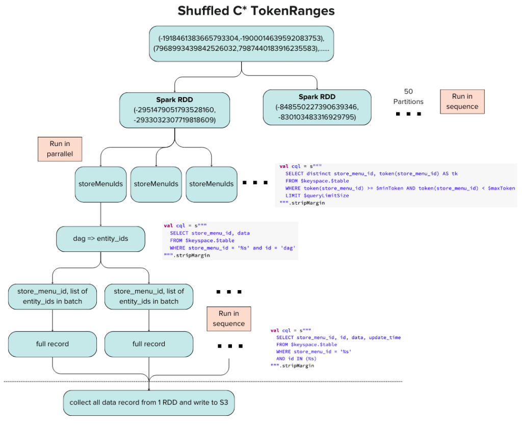
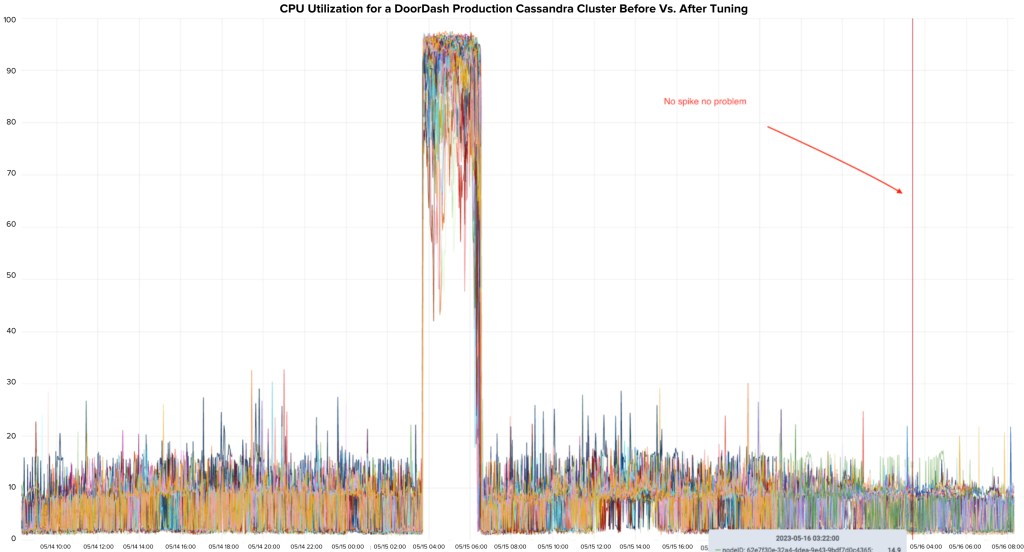
In one of our Cassandra clusters, we used its read-only DC to house expensive analytics queries that effectively take a daily snapshot of the tables. Because we treated the RO DC as complicated and isolated, as the number of tables grew the queries got more and more expensive. Eventually, the analytics job caused the RO DC to become pegged at 100% every night. This also started to impact the main DC. Working with the product team, we drastically optimized those batch jobs and created a better way to take the snapshot. Without going into too much detail, we utilized toke range to randomly walk the ring and distribute the load across the clusters. Figure 4 below shows the rough architecture.
Figure 4: Random walk daily scan architecture
The end result was amazing. The CPU spike was eliminated, enabling us to decommission the RO DC altogether. The main DC performance also noticeably benefited from this.
Figure 5: Optimized random walk for RO DC
GC tuning: Sometimes worth it
Within Cassandra, GC tuning, or garbage collection tuning, is a challenging task. It demands a deep understanding of garbage collection mechanisms within the Java Virtual Machine, or JVM, as well as how Cassandra interacts with these systems. Despite its complexity, fine-tuning the garbage collection process can yield significant performance improvements, particularly in high-throughput environments like ours at DoorDash. Here are some common considerations:
Prefer more frequent young generation collections: In JVM garbage collection, objects are first allocated in the young generation, which is typically smaller and collected more frequently. Tuning Cassandra to favor more frequent young gen collections can help to quickly clear short-lived objects, reducing the overall memory footprint. This approach often involves adjusting the size of the young generation and the frequency of collections to strike a balance between reclaiming memory promptly and not overwhelming the system with too many GC pauses.
Avoid old generation collections: Objects that survive multiple young gen collections are promoted to the old generation, which is collected less frequently. Collections in the old generation are more resource-intensive and can lead to longer pause times. In a database like Cassandra, where consistent performance is key, it’s crucial to minimize old gen collections. This can involve not only tuning the young/old generation sizes but also optimizing Cassandra’s memory usage and data structures to reduce the amount of garbage produced.
Tune the garbage collector algorithm: Different garbage collectors have different characteristics and are suited to different types of workloads. For example, the G1 garbage collector is often a good choice for Cassandra, as it can efficiently manage large heaps with minimal pause times. However, the choice and tuning of the garbage collector should be based on specific workload patterns and the behavior observed in your environment.
Monitor and adjust based on metrics: Effective GC tuning requires continuous monitoring and adjustments. Key metrics to monitor include pause times, frequency of collections, and the rate of object allocation and promotion. Tools like JMX, JVM monitoring tools, and Cassandra’s own metrics can provide valuable insights into how GC is behaving and how it impacts overall performance.
Understand the impact on throughput and latency: Any GC tuning should consider its impact on both throughput and latency. While more aggressive GC can reduce memory footprint, it might also introduce more frequent pauses, affecting latency. The goal is to find a configuration that offers an optimal balance for your specific workload.
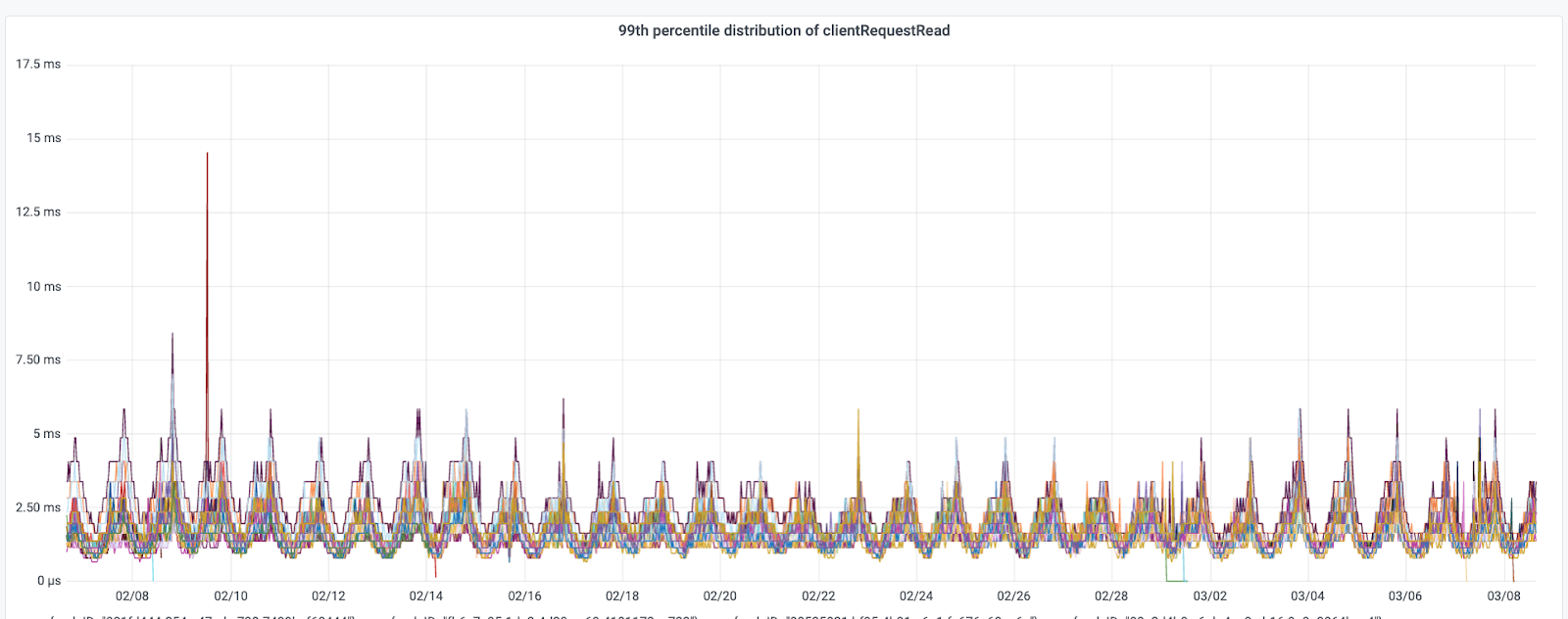
In our experience at DoorDash, we’ve found that targeted GC tuning, while complex, can be highly beneficial. By carefully analyzing our workloads and iteratively tuning our GC settings, we’ve managed to reduce pause times and increase overall system throughput and reliability. However, it’s worth noting that GC tuning is not a one-time task but an ongoing process of observation, adjustment, and optimization. Figure 6 below shows provides an example of when we tuned our GC to achieve better P99 performance.
Figure 6 : Latency improvement via GC tuning
Future work and applications
As we look toward the future at DoorDash, our journey with Apache Cassandra is set to deepen and evolve. One of our ongoing quests is to refine query optimizations. We’re diving into the nuances of batch sizes and steering clear of anti-patterns that hinder efficiency.
Another challenge remaining is performance of the change data capture, or CDC. Our current setup with Debezium, paired with Cassandra 3, suffers from limitations in latency, reliability, and scalability. We’re eyeing a transition to Cassandra 4 and raw clients, which offer better CDC capabilities. This shift isn’t just a technical upgrade; it’s a strategic move to unlock new realms of real-time data processing and integration.
Observability in Cassandra is another frontier we’re eager to conquer. The current landscape makes it difficult to discern the intricacies of query performance. To bring these hidden aspects into the light, we’re embarking on an initiative to integrate our own proxy layer. This addition, while introducing an extra hop in our data flow, promises a wealth of insights into query dynamics. It’s a calculated trade-off, one that we believe will enrich our understanding and control over our data operations.
Acknowledgements
This initiative wouldn’t be a success without the help of our partners, the DRIs of the various clusters that were tuned, including:
Ads Team: Chao Chu, Deepak Shivaram, Michael Kniffen, Erik Zhang, and Taige Zhang
Order Team: Cesare Celozzi, Maggie Fang, and Abhishek Sharma
Audience Team: Edwin Zhang
Menu & Data Team: Yibing Shi, Jonathan Brito, Xilu Wang, and Santosh Vanga
Thanks also to Levon Stepanian for helping track cost savings across AWS Infra and Instaclustr management fees. Finally, thank you for the support from the broader storage team and our Instaclustr partners.
DoorDash has grown from executing simple restaurant deliveries to working with a wide variety of businesses, ranging from grocery, retail and pet supplies. Each business faces its own set of constraints as it strives to meet its goals. Our logistics teams — which range across a number of functions, including Dashers, assignment, payment processes, and time estimations — seek to achieve these goals by tuning a variety of configurations for each use case and type of business.
Although that process started with a limited set of configurations, the old system struggled to keep up with DoorDash’s growth across new verticals. The assignment team alone hosts multiple files in GitHub to maintain the burgeoning number of preferences, some of them now weighing in at more than a megabyte each. It doesn’t help that these preferences aren’t kept in standard formats; some are JSONs, others are CSVs, and still others have no format at all. Maintaining these files and updating them at the speed of DoorDash’s growth has been both challenging and risky, with multiple outages occurring because of incorrect configurations. Additionally, the current system operates with a limited set of features, reducing the speed with which new capabilities and experiments can be launched.
With all of that in mind, we set out to build a new logistics configuration platform that could not only meet today’s demands but could continue to scale well into DoorDash’s future growth.
Current architecture
Figure 1: High-level assignment architecture
Figure 1 represents a simplified, high-level version of DoorDash’s existing architecture in which users update their preferences in GitHub files, which are then pushed to the Redis cluster. At delivery creation, KafkaConsumer reads the data from Redis, creates a delivery assignment constraint (DAC) object, and then stores it in a DAC table via delivery service. During the assignment run, DeepRed fetches this information from delivery service via Apollo and uses these configurations for an assignment decision.
Challenges and limitations
At a high level, there are some challenges and limitations in the current architecture, including:
Updating preferences in a single line for thousands of stores: DoorDash and its business partners operate in multiple countries and regions, each with its own specific preferences. For assignment purposes, preferences are set at various granular levels — business level, SP level, store level, and so on — resulting in a huge file of preferences. In the current implementation, there are thousands of stores that share the same preferences, creating a single line with thousands of stores. Adding, removing, or changing any of these generates a massive pull request, which is arduous to review and poses a significant risk of implementation failure.
Unintentional preferences:Given a single block of stores that has multiple preference types, there have been occasions when preferences have been updated unintentionally.
Difficult auditing and versioning: Although GitHub provides version control, proper auditing is impeded by heavily updated config changes in the same line.
Time-consuming process to add new preferences: DeepRed considers a lot of signals and preferences during delivery assignments. New businesses constantly introduce additional requirements, and those new preferences need to be added in multiple systems. In the current architecture, These preferences are in the DAC table, KafkaConsumer, Apollo, delivery service, upstream clients (which set the preferences), and then DeepRed, creating a process that can take up to a week.
There are also some lower-level limitations and missing capabilities in the current architecture, including:
No way to add ephemeral configs to run experiments: At DoorDash, we believe in running plenty of experiments to get the right values for all of our stakeholders. Ideally, we would like to run experiments on ad hoc configurations, but there is no way currently to add them temporarily and in a scalable manner.
Preferences are not real-time: When a delivery is created, corresponding DACs are also made; DeepRed must consider these additional constraints during the assignment process. Each DAC is created only once, so if certain preferences have been modified before DeepRed picks up the object, these new preferences are never considered for assignment. This is particularly troublesome for scheduled deliveries and also causes headaches during debugging. There have been multiple incidents when delivery was created before the new preferences could be set.
No single source of truth: DACs are pre-set at the business or entity level, but dynamic preference updates also are needed at the delivery level. Instead, DACs are updated via order service during order creation, but there is no way to know whether those preferences were created by order service or if they came from predefined values.
Incorrect usage of existing preferences: Because of the effort required to include new preferences, sometimes existing preferences with magic values are used to achieve certain outcomes.
Resolving issues with a logistics configuration platform
To address all of these challenges, we built a logistics configuration platform that provides a single source of truth with reliability, scalability, auditing, and improved velocity. We have included an intuitive UI — LxConsole — on top of the platform. Each configuration at a high level is independent, versioned, and both history- and approval-controlled.
Solving existing problems
Our new architecture sharply reduces the time needed to add a new preference type; what used to take more than a week can be done in less than a day. Additionally, auditing and version control are streamlined, with each config request resulting in a newer version entry in the database. By default, each configuration is created in an in-review state. Relevant stakeholders can then review the request and approve or reject it. This process provides a much clearer auditing path, showing who changes what, when, and why. The new architecture presents each request on a separate line, as shown in Figure 2 below, allowing the reviewer to see both the requested value and the older value. The first graphic in Figure 2 shows the impenetrable results built into our old system.
Before
These are partial screenshots of the git-diff results from a request to update two store configurations:
After
Figure 2: Results from submitting a request to update config for two stores.
Building new capabilities
Apart from solving existing problems, the platform comes with many new capabilities:
Expiration-based configuration: DoorDash has many use cases that need to set configurations for a certain time, and then auto revert them. This reduces time and effort to manage configuration and also avoids forgetting to revert.
Time-based preferences: Each business and vertical wants different settings at different times of day. In this new platform, businesses can submit preference values for each time window; the platform then can return values based on those times (considering various time zones). This saves a client the effort of storing each configuration and then parsing complex time and date handling on their end. Clients, instead, can simply submit their preferences and get appropriate results. With this, businesses can fine-tune their preferences to achieve better results, as shown in this example:
Time Window based configuration:
{
    { StartTime: “0”, EndTime: “10”, value: “10”}
    { StartTIme: “11”, EndTime: “23”, value: “20”}
}
Ephemeral config types: Many DoorDash teams run experiments on preferences, but not all experiments result in final configuration. So, we need a way to add ad hoc config-types to run experiments without bloating them because config-types are primarily for long-term preferences rather than short-term experimental preferences. We included support in the new platform for adding new preferences — ephemeral configs — which would not require dev effort. It used to take around two weeks to do this, but the new configurations now allow teams to launch experiments in less than a day.
Validation: Currently, there is no validation logic for different preferences. The new platform, however, does validations and rejects requests automatically if they do not satisfy predetermined criteria. This saves significant time for both the requester and the approver.
Auto approval/rejection: As we onboard more use cases with a high frequency of updates and certain validations in place, we can skip manual approval for certain requests. At a very high level, the new platform will do auto-approval in two cases:
Type-based auto approval/rejection: In these cases, all requests for a certain config type would be automatically approved. We are starting this with store-capacity, which are frequently updated configs by operators to adjust dispatch.
Rule-based auto approval/rejection: In some cases, we can approve a request automatically when certain conditions are satisfied. For example, if validation for a given configType is successful and submitted by a certain group of people, the system can automatically approve the request.
Extendable to any configuration type: With JSON as a type, the client theoretically can submit any arbitrary configuration and start using it in less than a day. The new platform does basic validations for JSON type and can add additional validations based on config-type. The platform is extensible so that any business can come and add their own validations on top of basic validation. With this design, clients can start using config-platform immediately and can also add additional support when needed.
Experiment-based configuration: Engineers can set up their experiment configuration easily and write a JSON blob with required metadata such as experiment name, control, and treatment values as shown here:
requester/approver/creationDate/description: other metadata
Explanation
Domain: namespace (Pay, Assignment, Dx etc)
entityType: store, business, SP, Delivery (more to add)
entityId: <ID based on type>
configType: <predefined type>
version: Auto increment with each request
Example
domain
entity_type
entity_id
config_type
version
config
config_status
created_at
expires_at
created_by
Pay
Store
12345
TEST_CONFIG
1
7
APPROVED
2023-06-20 19:22:04
saurabh
Figure 3: Example of a stored record
Extendable to any entity type: As mentioned above, DoorDash works at various levels of granularity. This new platform supports adding configurations at all levels.With the schema shown in Figure 3 above, the platform can set configurations at any entity level. For example, if tomorrow there is a need to set a preference at a state level, users can simply add it with no need to make any changes except updating enums, which controls what’s coming into the system. As with other parts of the design, this data model was finalized after multiple iterations. So far, this has worked for all foreseeable use cases.
Stay Informed with Weekly Updates
Subscribe to our Engineering blog to get regular updates on all the coolest projects our team is working on
Please enter a valid email address.
Thank you for Subscribing!
Lessons learned
This section encapsulates our fundamental takeaways, providing a snapshot of the insights gained from our existing architecture and our transition to the new platform. These key lessons set the stage for the pragmatic yet forward-thinking approach we’ll adopt in the upcoming steps, ensuring a robust foundation for the journey ahead.
Think big, start small: This was a key development strategy for the platform from Day One. When we started the project, we were uncertain about the capabilities and client requirements that would be included. Instead, we focused on a basic concept: Build rock-solid small components and then iterate on top of them.
Latency: We started with a basic CockroachDB cluster (CRDB) and three Kubernetes PODs per cell. This gave us enough performance to achieve our minimum viable product goals. We started with 300 queries per second (QPS) with p99 <10 ms; all of these were non-batched requests. As we started onboarding additional use cases and traffic, latency increased. We had to identify and fix a few problems to get latency back to where we wanted it.
The first bottleneck we hit was when we opened traffic for batched calls from the snapshotting stage. Our latency shot from <10 ms to 500 ms for those batch calls. We moved from the default coroutine dispatcher to io-dispatcher, which increased parallelism. This improved our latency for batch calls from 550 ms to 350 ms, which was sufficient for our use case. Nonetheless, we continued to pursue improvements.
Upon further analysis on the client side, we realized that we were supposed to create small batches; because of a small bug, however, we were making a single call with 2000 IDs rather than a batch size of 100 and we were contending with some duplicate IDs. Once we resolved these issues, our latency dropped from 350 ms to 40 ms.
This batch call was gated behind the feature flag, which was enabled only for a subset entity types and corresponding entity ids. As we opened all traffic to config-service, our latency increased again from 40 ms to roughly 700 ms. We upgraded our CRDB cluster’s instance-type which improved latency from 700 ms to 450 ms.
We dove deeper to continue pursuing latency improvements. Though QPS to config-service didn’t increase much – 350 to 500 but peak QPS from config-service to CRDB increased from 400 req/sec to 20,000 req/sec. This was because, 1 single bulk-query request (with 1000 entities) was divided into individual request to CRDB (1000 request). After we changed our query from = clause to IN clause to use multiple entity ids, latency came back to a normal range of around 40 ms and had the same QPS to config-service and CRDB (Figure 4).
Figure 4: Latency Improvement
Integration tests and local testing: Even before launching our MVP,we built integration tests and local testing setups into our system which helped in catching bugs and doing local testing at every stage. This also helped us build our iteration with confidence.
Decoupled components and query patterns:Although we built a single endpoint for all retrieval use cases, we built use case-specific handlers. This gave us:
Separate queries for separate use cases: Based on use cases, we optimized our queries repeatedly; updating a query for one use case didn’t interfere with other queries.
Flexibility to move multiple endpoints: This also gives us the flexibility to break our single endpoint into multiple endpoints based on use cases without making any changes in our internal handlers. An example of this would be creating separate endpoints for UI versus service calls.
Use out-of-the-box solutions when available: It’s always best to deploy any available out-of-the-box solutions. DoorDash’s internal platform team already has built many features which come in handy, like an Asgard-based microservice, which comes with a good set of built-in features like request-metadata, logging, and dynamic-value framework integration.
Migration challenges
Our biggest challenge has been to migrate existing preferences even as the old system is actively being modified. With multiple stakeholders continuing to update the existing GitHub, it has been difficult to maintain parity with the new system. From the start, we adopted a few best practices to streamline the process, including:
Good parity framework and migration scripts:We built a parity framework to compare results between the platform and runtime. Running in real-time, this framework can generate logs and metrics if there are any differences between the two systems. It also has helped in switching from using old preferences to new preferences with a small configuration.
Scripts: Scripts helped us to convert to the final format — CSV — saving us a significant amount of time.
Clear guide with sample files and tracker: We prepared a guide and tracker to maintain clarity on which configurations already had been migrated, which were in progress, and how to prepare data for each config type.
Communication: Maintaining clear communication at every level has been vital. We have proactively communicated with our stakeholders about what’s been launched, what remains a work in progress, how to use the new platform, and where to find any additional information they might need. We also monitor any changes being made in GitHub so that we can immediately ask stakeholders to use the new tool. This provides two advantages: No parity errors and immediate partner onboarding.
Next steps
Now that we’ve examined what we’ve learned from our existing architecture let’s shift focus to what lies ahead. The new architecture, called LxConfig Platform, allows us to pursue many new advantages, including:
More clients and use cases: We recently launched our MVP and are excited to add more features to it. The LxConfig Platform has become a central focus for a variety of goals that we have set for next year and beyond. The platform is becoming a de facto standard to store the configurations. Our initial users were on the assignments team, and we are actively working on to onboard new teams, like pay, ETA, Drive.
Simplified architecture: As previously noted, we are working towards simplifying the assignment system architecture by removing a number of unnecessary components as shown in Figure 5 below:
Figure 5: New architecture
Scaling: We currently are handling 500 req/s with less than 10 ms latency (p99) for non-batch calls and 40 ms for batched calls. As we bring on more clients and use cases, we need to increase this to 10,000 req/s while keeping latency as low as possible.
Rules-based configuration: Just as with the different configurations required for varying time designations, certain conditions also require specific configurations. Currently, the client must build custom logic and do the processing. With rule-based configuration, however, clients can set configurations with discrete rules when they submit the request. At retrieval, the user can opt to pass a filter parameter, which the platform can use to return different values, as shown below:
Permission model design: Only the platform team currently has permission to approve requests, which is not a scalable solution for the long term. First, the platform team doesn’t have insights about the type of changes being requested. Second, approvals would consume far too much bandwidth from platform team engineers. While we work with the identity and security team to build a sophisticated permissions model, we are developing our own config type-based model to expand the set of people able to approve certain requests.
Optimization: We are maintaining an ongoing search for hot spots in logic and query that could be improved over time.
Reliability: We are careful to set realistic expectations for this new platform as we bring in clients and use cases. We are still building resiliency into our system by adding more endpoints to our SLO targets, fine-tuning our metrics, and building our infra resources, among other efforts. We continue to work toward building this platform’s ability to support T0 services and hard constraints. All current platform clients are T0 service, have fallbacks in place, and can perform in a degraded fashion if the platform becomes unavailable.
Async request processing: The current platform can handle about 30,000 rows of CSV file processing in roughly one second in a sync call. This needs to increase when we begin to onboard daily update configurations that can include up to 100,000 rows. This can be achieved synchronously through finding and improving current limitations, keeping latency within one second, or asynchronously through decoupling request submission and processing. Moving to asynchronous will provide additional functionality and several advantages, including:
Building a better write-path framework, breaking bigger requests into smaller parts;
Allowing for partial success and failure and providing users details about success/failure.
Scaling at very high input; and
Easing the handling of system-submitted requests.
New endpoints: Currently, requests are submitted only through LxConsole. As we move to support use cases in which configs are updated dynamically based on order type or through ML models, however, we need better methods for storing those requests. Having separate endpoints for them will keep the blast radius limited and isolated.
New input formats: Currently, the platform is supporting byte-based input. We want to move to other formats, including file-based and record-based.
Easy migration: With many configurations spread across multiple locations in a variety of formats, we need to improve ways to move them to config-service. Currently, we are exploring converting them to the format required by config platform if those configs are generated by a system that can be updated to use a new format. Alternatively, we can build a framework within config platform to consume CSVs and create JSONs out of them automatically. This process is ongoing while we determine which option will work best.
Auto-consuming: While config platform is fed the data manually at the moment, we want to build a system for certain use cases to allow the platform to periodically check and pull the configuration from an auto-generated system, including possibly an ML model-generated configuration.
Raw and derived configuration: We are also building capabilities to store raw and derived configuration data in config service for consumption and analytics. Details are being discussed, but we are excited to pursue this idea.
Improving developer and partner velocity: While we have a good local testing framework at the moment, there are times we need sandboxes for doing end-to-end testing. We plan to enhance our platform with sandboxes that are in line with the rest of DoorDash. This will let developers spawn new environments and conduct end-to-end testing faster.
Improved testing environment: Currently, LxPlatform doesn’t have a test endpoint. Because of this, clients connect to the prod environment for their testing. Depending on the number of clients, this could significantly increase QPS. We are considering building a parallel non-prod environment for end-to-end testing without affecting prod.
Refine data model: As more use cases come in, we want to maintain a level of control while also allowing some flexibility regarding what kind of data to store. In the current model, configType is a single value, but we are exploring breaking it into two levels: configType and configSubType. With this change, a certain config type can have unlimited subtypes without needing to update enums for new subordinate use cases.
Data warehouse pipeline: We are working to set up a pipeline to move data from the primary database to a data lake for long-term storage, providing easy accessibility for analytics. This will help keep the primary database small, providing better performance.
Self-serve new config type registration: A lower-priority goal would be to provide a self-service option for partners to define their own config types. All the properties defined for these config types would be part of the registration process. This would free the platform from having to add any code changes for new config types.
Final thoughts
We started with a big vision and continue to move in that direction one step at a time, learning as we go along. Creating the platform was just the beginning. We are excited about the possibilities for continued growth as we continue to iterate and improve the system to meet the ever-changing needs of DoorDash’s growing business.
If you’re passionate about building innovative products that make positive impacts in the lives of millions of merchants, Dashers, and customers, consider joining our team.
Acknowledgements
Thank you to the working group, Ben Fleischhacker, and Ashok Thirumalai for their contributions to the discussion, design, and execution. Thanks to Paul Brinich and Gayatri Iyengar for your constant leadership support on the project. Thanks Sameer Saptarshi, Suhas Khandiga Suresh, and Ryan Xie for working both as partners & contributors. Thanks Joy Huang and Lillian Liu for reviewing product perspectives.
Finally, many thanks to Janet Rae-Dupree, Robby Kalland, and Marisa Kwan for their continuous support in reviewing and editing this article.
There have been many benefits gained through DoorDash’s evolution from a monolithic application architecture to one that is based on cells and microservices. The new architecture has reduced the time required for development, test, and deployment and at the same time has improved scalability and resiliency for end-users including merchants, Dashers, and consumers. As the number of microservices and back-ends has grown, however, DoorDash has observed an uptick in cross-availability zone (AZ) data transfer costs. These data transfer costs — incurred on both send and receive — allow DoorDash to provide its end users a highly available service that can withstand degradations of one or more AZs.
The cost increase prompted our engineering team to investigate alternative ways to provide the same level of service more efficiently. In this blog post, we describe the journey DoorDash took using a service mesh to realize data transfer cost savings without sacrificing service quality.
DoorDash traffic architecture
Before we dive into our solution, let’s review DoorDash’s traffic infrastructure.
Cell-based architecture: As shown in Figure 1 below, our traffic architecture follows a cell-based design. All microservice pods are deployed in multiple isolated cells. Every service has one Kubernetes deployment per cell. To ensure isolation between cells, intercellular traffic is not permitted. This approach enables us to reduce the blast radius of a single-cell failure. For singleton services or those not migrated to the cell architecture, deployment occurs in a singular global cell. Internal Envoy routers allow communication between the global cell and replicated cells.
Kubernetes cluster deployment: Each cell consists of multiple Kubernetes clusters; each microservice is deployed exclusively to one cluster within a given cell. This design ensures scalability and reliability while aligning with our cell-based architecture.
Figure 1: Cell-based multi-cluster deployments
High availability: To enhance availability and fault tolerance, each Kubernetes cluster is deployed across multiple AZs. This practice minimizes disruptions caused by an outage of one or more AZs.
Direct communication in a flat network: Leveraging AWS-CNI, microservice pods in distinct clusters within a cell can communicate directly with each other. This flat network architecture streamlines communication pathways, facilitating efficient interactions between microservices.
Custom multi-cluster service discovery: Our custom service discovery solution, DoorDash data center Service Discovery, or DDSD, provides a custom DNS domain to support multi-cluster communication. Clients leverage DNS names to dynamically discover all pod IP addresses of desired services. DDSD’s functionality is similar to Kubernetes headless services, but it works for inter-cluster communication as well. For instance, a client in a different cluster can use payment-service.service.prod.ddsd to retrieve all pod IP addresses associated with the payment service.
Client-side load balancing: Service mesh is responsible for client-side load balancing. For services not onboarded to service mesh, however, load balancing occurs on the client application side.
Figure 2 depicts the four characteristics outlined above:
Figure 2: Intra-cell and cross-AZ communication patterns
Service mesh architecture: DoorDash’s service mesh as outlined in Figure 3, which is deployed to each cell, adopts a sidecar container design pattern, leveraging Envoy proxy as the data plane. We’ve built our own xDS-based control plane to manage Envoy configurations. The sidecar container operates as a plug-and-play solution, seamlessly intercepting, controlling, and transforming all HTTP1/HTTP2/gRPC traffic flowing in and out of DoorDash microservices — all without requiring any modifications to the application code.
Figure 3: Service mesh high-level architecture
While DoorDash’s traffic architecture has unique components, we believe the challenges and lessons we’ve encountered on our network traffic-related efficiency journey can be applied broadly to other architectures as well.
Common DoorDash data transfer patterns
For cross-AZ traffic, we categorize our traffic patterns as follows:
HTTP1/HTTP2/gRPC traffic: Direct pod-to-pod communication between microservices within the same cell; the traffic between microservices in the global cell and those in cells that involve an additional hop in the call path — such as internal routers — increases the likelihood of cross-AZ traffic.
Storage traffic:Includes traffic from microservices to stateful systems such as Aurora PostgreSQL, CockroachDB, Redis, and Kafka.
Internal infrastructure traffic:Internal Kubernetes traffic such as coredns traffic or communication between Kubernetes control plane components. This type of traffic usually uses Kubernetes internal DNS instead of DDSD.
Early hypothesis
We believed that HTTP1/HTTP2/gRPC traffic within the same cell was the largest source of cross-AZ data transfer costs because of our microservice architecture. We also determined that service mesh potentially could enable zone-aware routing for all microservices using that feature in Envoy. Understanding both of these things, we prioritized investigating and optimizing HTTP1/HTTP2/gRPC traffic patterns to improve efficiency without degrading service quality.
Addressing HTTP1/HTTP2/gRPC traffic costs
Originally, traffic between services was uniformly distributed across different AZs as shown in Figure 4. With Envoy’s zone-aware routing feature, caller services now prefer directing traffic to callee services in the same AZ, as shown in Figure 5, thereby reducing cross-AZ data transfer costs.
To enable Envoy’s zone-aware routing feature, we made changes in our control plane for service mesh, switching the service discovery type from STRICT_DNS to endpoint discovery service (EDS). As shown in Figure 6 below, for DDSD domains, the control plane now dynamically sends EDS resources from each Envoy cluster back to Envoy sidecar containers. The EDS resource includes pod IP addresses and their AZ information.
With the data provided in EDS responses, Envoy retrieves the AZ distribution of both the caller service and the callee service. This information enables Envoy to calculate weights between pods. Although sending traffic via local AZs is still prioritized, some traffic may still be directed across AZs to ensure a balanced distribution and to avoid overloading any single pod as shown in Figure 7.
Figure 7: Preferring local AZ while ensuring balanced traffic
This routing solution offers several benefits, including:
Maintaining traffic balance, even in scenarios where services are unevenly distributed across AZs
Making it possible to dynamically set traffic weights between pods, eliminating manual operation
Reducing the blast radius of a single or multi-AZ outage
Reducing traffic latencies — caller services connect to callees that are more proximal
Our solution becomes even more effective when service pods are evenly deployed across AZs. To achieve this, we leveraged topologySpreadConstraints and set maxSkew to 1 with whenUnsatisfiable: ScheduleAnyway as shown in Figure 8. This means the Kubernetes scheduler will still schedule pods even without the condition being satisfied, prioritizing nodes that minimize the skew.
This approach ensures that pods are still scheduled; not doing so would reduce the amount of bin-packing, increasing idle compute and ultimately eating into zone-aware traffic-related cost reductions. In our production system, we observe 10% of traffic that is sent across AZs with this topologySpreadConstraints policy.
Figure 8: Configuration to deploy pods evenly across AZs
As we gradually rolled out the above changes, we saw improvements in our AWS cross-AZ transfer charges. Even so, we expected larger reductions. So, we set about investigating why we weren’t saving as much as we had anticipated.
Stay Informed with Weekly Updates
Subscribe to our Engineering blog to get regular updates on all the coolest projects our team is working on
Please enter a valid email address.
Thank you for Subscribing!
Finding the needle in the haystack: Better visibility into cross-AZ traffic
We confirmed zone-aware routing was working as expected by validating Envoy metrics between AZs and logs from applications, but we needed more visibility into cross-AZ traffic to determine the root cause of the lower-than-expected reduction in data transfer costs. This led us to use a number of observability tools, including VPC flow logs, ebpf agent metrics, and Envoy networking bytes metrics to rectify the situation.
Using VPC flow logs, we mapped srcaddr and dstaddr IP addresses to corresponding subnets that were deployed in our AWS account structure. This mapping provided a roll-up rule that let us make sense of overall egress/ingress traffic patterns between different subnets hosting various parts of our cloud footprint, including subnets for production Kubernetes clusters, storage solutions, caches, and message brokers as shown in Table 1. We were able to confirm that our largest source of cross-AZ transfer costs is non-storage traffic within each cell. Around 20% of this cost was caused by traffic to one elastic load balancer (ELB) used for our event ingestion pipeline (Iguazu).
Table 1: Cross-AZ traffic attribution using VPC Flow logs
Additionally, we examined service mesh HTTP1/HTTP2/gRPC metrics, specifically connection bytes for all requests and responses for both ingress and egress traffic. The most important metrics from service mesh Envoy proxy are cx_rx_bytes_total and cx_tx_bytes_total from both Envoy listeners and clusters. However, because not all services were onboarded to service mesh at the time, we relied on metrics from BPFAgent, which is globally deployed on every production Kubernetes node, to increase visibility into total network bytes. Using metrics from both of these sources, we discovered that 90% of all traffic is HTTP1/HTTP2/gRPC traffic; 45% of that traffic had already been onboarded to service mesh and 91% of that portion of traffic is being sent to Iguazu!
Hops after hops: Iguazu’s traffic flow
After analyzing Iguazu’s traffic flow as shown in Figure 9, we realized there were several intermediary hops between the caller and callee services, or pods. When traffic moves from the caller services to Iguazu, it initially passes through ELBs, before landing on one of the worker nodes in a different Kubernetes cluster in the global cell. Because the externalTrafficPolicy is configured as a cluster, iptables redirects the traffic to another node to ensure load balancing.
Figure 9: Iguazu’s original traffic flow
We observed the following data transfer behavior:
Clients who were sending traffic to ELBs were still using the ELB DNS names directly. Because clients were not using the internal DDSD domains, the service discovery type in the Envoy cluster was still STRICT_DNS instead of EDS, which is a prerequisite for enabling zone-aware routing. This meant the Envoy sidecar containers used a simple round-robin approach to distribute traffic to the ELBs.
Cross-AZ load balancing was disabled in the case of traffic from ELBs to Kubernetes worker nodes in Cluster 2.
When traffic arrives at a Kubernetes worker node from the Iguazu ELB, it is subsequently redirected by iptables to a random node, which also increases the probability of cross-AZ traffic.
Given the complexity of multiple hops within the Iguazu call graph, we decided it would be best to migrate the Iguazu service to the same cell where their clients were deployed.
We also configured the routing rules of all clients’ Envoy sidecars to route traffic to Iguazu pods in the new cluster instead of talking to the ELBs — without requiring our engineers to make any code or config changes to their services. This allowed us to enable direct pod-to-pod communication for Iguazu traffic, enabling zone-aware routing while simultaneously reducing the volume of traffic processed by the ELBs as shown in Figure 10.
Figure 10: Iguazu’s new traffic flow
These actions made such a material dent in DoorDash’s data transfer costs as well as our ELB costs that it caused our cloud provider to reach out to us asking whether we were experiencing a production-related incident.
Lessons learned
Some of the key discoveries made during our journey include:
Cloud service provider data transfer pricing is more complex than it initially seems. It’s worth the time investment to understand pricing models in order to build the correct efficiency solution.
It’s challenging to build a comprehensive understanding/view of all cross-AZ traffic. Nonetheless, combining network bytes metrics from different sources can be enough to identify hotspots that, when addressed, can make a material dent in usage and cost.
Envoy’s zone-aware routing can send traffic to its local availability zone while automatically ensuring resiliency through balanced traffic.
As the number of hops increases in microservice call graphs, the likelihood of data being transmitted across AZs grows, increasing the complexity of ensuring that all hops support zone-aware routing.
If you’re considering a service mesh for its traffic management features, you may also leverage it for greater efficiency.
To learn more about DoorDash’s service mesh journey, check out Hochuen’s KubeCon + CloudNativeCon North America 2023 service mesh session.
Future work
We’ve already compiled a list of solution enhancements we’d like to implement, including:
Streamline the process to gather metrics from different sources and provide a unified overview of cost and usage.
Enable the zone-aware routing feature for internal Envoy routers
Make the solution more extensible to support HTTP1/HTTP2/gRPC traffic using other domains beyond DDSD.
Enable the topology-aware routing feature for internal infrastructure traffic using the Kubernetes network proxy kube-proxy.
Explore optimized routing for large data transfer operations to or from DoorDash’s stateful systems, for example PostgreSQL, CRDB, Redis, and Kafka. This will allow traffic to remain in single AZ swim lanes whenever it makes sense, further reducing costs.
Acknowledgement
We thank Darshit Gavhane and Allison Cheng for migrating all Iguazu services to the same cell where clients are running, as well as Steve Hoffman and Sebastian Yates for their advice and guidance along the journey.