Skip to content

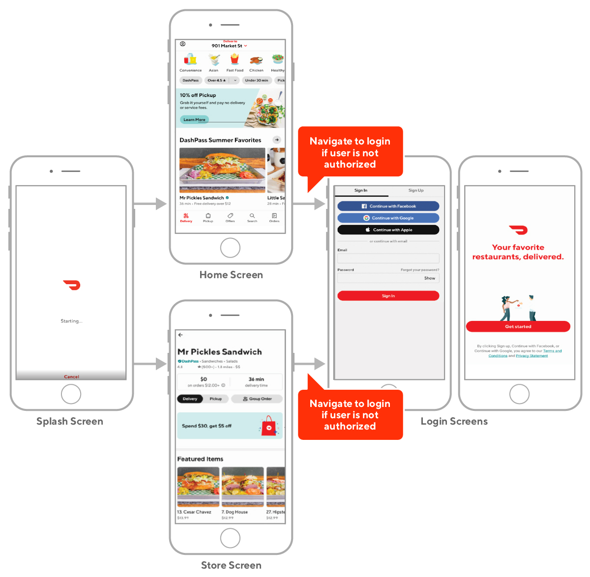
When DoorDash added a pickup option for customers, complementing our existing delivery service, we needed to build a map to ensure a smooth user experience. A map tailored to pickup users could show nearby restaurant options, enabling customers to factor in distance to their selection process. 

We successfully implemented such a map in our mobile app and saw positive results from our customers, indicated by increased conversion rates. We wanted to replicate that success for the DoorDash web experience, giving our customers yet another option when ordering.

However, when implementing a pickup map for our web experience, we encountered a number of challenges. To maintain performance and a rich featureset, we needed to carefully design its underlying architecture and APIs. Unlike mobile apps, geolocation is not a given for web applications, so we had to make some important choices around determining the customer’s location. 

Designing a pickup map for DoorDash

When DoorDash added a pickup option to our web experience, we wanted to build a map to improve the user experience (UX), which had been a successful feature on our mobile app. A pickup map displays all the restaurants near the customer’s current location and includes a carousel for recommendations. DoorDash did not previously have a map because when our business was only deliveries, customers only needed the restaurant’s name and the estimated delivery time, which was best displayed as a list. 

When we introduced the pickup option, adding a map to our mobile app improved the UX because pickup users require information about restaurants’ locations relative to theirs. And beyond the functional aspect of showing a customer how to get to a restaurant, the map also lets customers browse for options nearby.

Figure 1: Our map for customers placing a pickup order lets them discover restaurants through their actual locations on the map and an associated list.

What we learned when implementing a pickup map at DoorDash 

Building a pickup map for the web experience has some technical complexities. Firstly, it required thorough design and planning to make it integrate with our web framework. Secondly, we had to make some technical choices on which location and map APIs to use. 

Lesson 1: Build a custom map library

Having our own map library allows us to future-proof the application, since it gives us the full control and flexibility we need to easily add new features and integrations. When integrating the Google Maps platform we considered many libraries to connect with React, our chosen frontend framework. These libraries could be used to save time and simplify the overall implementation. In the end, we decided to build our own map library, in order to optimize flexibility and performance. Building our own library gave us full control of the integration between the Google Map API and our React components, avoiding any potential limitations introduced by a third party library. 

Having our own library also ensures that future integrations and changes are smooth and easy to build. For example, we had planned to add a recommendation list in a carousel format after launching the initial pickup map. Since we had built our own library, we were able to move fast without having to make any trade-offs or hacky decisions.

A custom library also helps optimize performance by ensuring there are no extra unused features. While we plan on adding a lot of additional features, we also wanted to make sure that our application runs as smoothly and quickly as possible. Therefore we decided to build our own library since using a third party library means including many extra features, which we were not ready to use. 

For example, the only features we needed from the Google Maps API were click and hover interactions, which are not worth the performance cost of implementing the entire library. By building our own library we ensured that we only used the features that we needed, enabling us to optimize for performance. 

Lesson 2: Understand the pros and cons of using the Geolocation API

When designing the pickup map, we wanted to make sure that our customers would be able to search for restaurants based on their current location or delivery address. On the web, one of the best options to get a user’s current location is the Geolocation API from the browser. We chose the Geolocation API over other alternatives because it’s native to the browser, which means it won’t hurt the web app’s performance. Nevertheless, there are several pros and cons when it comes to the Geolocation API that will shape how to use it effectively.

Pros: 

Two of the main advantages of using the Geolocation API are its native browser support and  simple API interface. The Geolocation API is native to most browsers including Internet Explorer, which means no additional libraries need to be imported and there is no incremental overhead on the web app’s bundle size. This lack of overhead helps us optimize performance. 

Besides that, the Geolocation API has a pretty simple interface that makes it easy to integrate into the web app. We merely need to type navigator.geolocation.getCurrentPosition to start the API integration process. Writing a lightweight wrapper for whichever framework is being used is extremely simple as well. We wrote a hook to tie the Geolocation API usage to our React component life cycle in less than a day. Overall, the native browser support and the simple API interface are the main advantages of using the Geolocation API and main reasons why we chose it.

Cons:

However, the Geolocation API does have a few drawbacks. In some scenarios, it can be slow to retrieve locations. In addition, the API’s interface for prompting the user to grant permission to get their current location is not ideal. 

First, getting the user’s location through the Geolocation API can be slow depending on the region and connection speed. This slowness results in a blank screen until it’s received, which might result in a customer giving up on placing an order. 

However, it’s possible to disable the high accuracy mode from the Geolocation API, potentially resolving the blank screen problem. This high accuracy mode requires more resources on mobile devices, so by disabling it we will be able to get the user’s location more quickly. 

Second, the Geolocation API does not come with a great interface for prompting the user to give the web app permission to access their current location. When implementing features like the pickup map, it is usually required to know if the user has already given permission to get their location, so that the web app would use the correct location to initialize the search. 

Out of the box, the Geolocation API actually doesn’t have a method to simply retrieve the user’s permission state. In fact, the two main methods for getting locations initiates two actions: prompting users for their permission and fetching their current locations. These two actions cause some difficulties when separating permission management from getting locations.

One way to improve this poor user interface for getting permission to retrieve the user’s current location is to utilize the Permissions API. A native browser API, the Permissions API works better than storing the user’s permission data in local storage or cookies, which is a common way to solve the issue of the user’s permission state. 

However, the data stored in the browser can become outdated quickly. If the user manually changes their permissions, the data stored won’t be updated automatically. Instead, the Permissions API is designed to solve the permission problem by providing straightforward methods to query the user’s current permission status on any browser’s APIs including the Geolocation API. The use of the Permissions API will always return the correct status. Unfortunately, the Permissions API is not supported by Internet Explorer or Safari, which limits this method for a significant portion of users. 

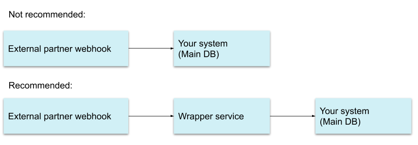
Lesson 3: Always include a fallback mechanism 

It’s essential to offer a fallback mechanism in case the Geolocation API returns an error, so that the user experience is not negatively impacted. Errors usually come from a denied permission request or from a timeout. In fact, it is recommended to always assume that users will block a permission request. 

For example, a fallback option could be the user’s default address in the system if the current location is not available. If the default address is not available either, another option is to derive a location from the user’s IP address. These fallback options ensure that we always have an address on hand to show restaurants nearby. In summary, assume users will not share their current location and plan the fallback experience accordingly.

Lesson 4: Make sure to plan out all interactions in detail

Because a map’s interactions and features can be quite complex, it’s important to plan all these out with a product manager and product designer to ensure success. Maps have a lot of edge cases. For example, what happens when two restaurant pins are very close, making it difficult to accurately select one? Figuring out all these edge cases in advance will prevent future bugs and ensure a more complete product. 

It’s also important to understand the technical limitations of each technology being used, since technical limitations restrict what can be built. Here are some examples we ran into: 

  • We could only conduct searches based on a set radius around a center point rather than within map boundaries. The map boundaries were rectangular but search results would only appear in a circle around the map’s center point, meaning that we either had to enlarge the map boundaries or exclude results in the corners of the map.
  • The Google Maps API does not support panning from point A to B if the distance between them is too large, instead jumping between the two points. This jump creates a jarring user experience, since the user would see a sudden change on the map without any context of where the change came from.
  • Out of the box, the Google Maps API does not have great support for styling label text. It only allows changes to basic styles such as the font family and font size, but not background color, which is very important for ensuring the visibility of overlapping label texts.

No matter what libraries are chosen, or even the in-house APIs, there are going to be some restrictions that will need to be dealt with. Technical limitations usually have an impact on not only the design, but also the product side as well. Therefore, it’s important to let all stakeholders know and make sure everybody agrees on the alternatives.

Conclusion 

Many companies need to improve user experience by building a user map to nearby services, and there are tons of ways to implement them. Every choice matters and has a profound impact on the product in the long term, so we think it is extremely important to choose what makes the most sense. Our lessons from the DoorDash pickup map project will help anyone build a similar map and decide which technologies to use, and make the best decisions based on their goals and needs.

Future work 

In the future, we are going to create different types of filters and searches for our pickup map. These would improve the UX by helping customers narrow down and find the restaurants they have in mind. We also intend to adopt the Permissions API to ensure the user’s permissions are as up to date as possible. The Permissions API would help bridge the gap between customers and our app on permission statuses. 

Furthermore, we aim to improve the web app’s performance by examining how the page components interact with each other, the backend services, and the map library. These optimizations would ensure that the customers can use our app seamlessly with any connection speed. 

Header photo by Thor Alvis on Unsplash

Experimentation lets companies such as DoorDash trial new features among a limited group of users to gauge their success. For example, we might try showing personalized restaurant recommendations in a grid format as opposed to a list format on our app. If data shows that our experimental group of customers like the grid format, we might roll that feature out to our entire user base. These experiments can also be performed in non-consumer facing aspects of the application. For example, we experiment on different algorithms for delivery assignments to Dashers and choose the best algorithm based on our internal metrics, such as delivery time (time taken to complete a delivery) or number of completed deliveries.

In an effort to derive the highest quality data possible from these experiments, we developed Curie, our new experimentation analysis platform. Curie standardizes our experimentation analysis processes and results, and makes the data accessible to all stakeholders. 

Built on a combination of SQL, Kubernetes, and Python for its main components, we named Curie after the famous scientist Marie Curie, honoring her experiments in radioactivity. Curie is designed to standardize our experiment analysis processes, including A/B tests, Switchback tests, and Diff-in-Diff analysis. This platform will help us make data-driven decisions based on the analysis results by validating the statistical significance (p-value) and treatment effects on metrics of interest.

Experimentation challenges before Curie

Prior to Curie, DoorDash’s data scientists analyzed their experiments in their local environment using SQL queries or ad-hoc scripts. This process was time consuming and error-prone. It also lacked standardization, as everyone used different methods for analysis, which can affect the quality and accuracy of the results. Lacking a centralized platform, experiment results were scattered in the form of documents or emails. 

Given the different types of experiments we ran and the scale at which our data was growing, it was difficult to find a single tool that catered to all our needs. We also wanted to leverage open source tools and integrate with our data and internal tools, including ACLs and workflows.

To address the above problems, we decided to build our own in-house experimentation analysis platform to enjoy all the benefits of automated analysis. We designed the platform to improve the accuracy of the experiment results by using standard and scientifically sound methodologies proposed by our experimentation working group. The analysis platform would also provide a centralized environment to showcase experiment results and make it easy to share them across the company. Experiment results would be precomputed and readily available so that the data scientists need not wait for the completion of long-running queries. 

The experiment life cycle at DoorDash

Before getting into the details of Curie, let’s first understand how it will be used during the life cycle of an experiment at DoorDash. As an analysis platform, Curie ingests data from experiments we have conducted and performs scientific analysis on the metrics, a process previously carried out by ad hoc scripts, as shown in Figure 1, below:

Diagram of DoorDash's experimentation methodology.
Figure 1: The life cycle of an experiment goes through multiple components of the experimentation platform, including configuration, instrumentation, and analysis.

The following sequence explains the life cycle of an A/B experiment randomized on users:

  1. The experimenter calculates the sample size required for an experiment by inputting their desired power and Minimal Detectable Effect (MDE). In this case, the sample size will be the number of users, as we are experimenting on users. In this step, the experimenter defines the allocation of the users among the control group (the users who do not see the new feature) and the treatment group (the users who are exposed to the new feature) based on a specific criteria, such as country or device type. Initially, we start with a small number of users in the treatment group and, depending on the preliminary results of the experiment, we gradually increase the treatment allocation until we completely allocate all the users to the treatment group. 
  2. The experimenter also sets up the experiment analysis configuration in the Curie web-based interface (WebUI). This configuration includes the list of metrics that need to be analyzed for this experiment. 
  3. When a user opens the DoorDash app, they will be randomly bucketed into either the control or treatment variation based on the allocation ratio specified in the first step. 
  4. This bucket assignment along with some contextual information (which we call experiment exposure events) are then logged in the data warehouse by our instrumentation infrastructure. 
  5. Curie performs the analysis using the exposures and metric data from the data warehouse and stores the results in the datastore.
  6. The analysis results will now be available on the Curie WebUI. The experiment will run for a period of time until we reach the required sample size. The experimenter can monitor the analysis continuously on Curie to confirm that the experiment does not have any negative effects on important metrics.

Curie’s components

Let’s now zoom into Curie’s architecture. Curie is an end-to-end system, where multiple components such as WebUI, workers, stats engine, and metric definitions collectively function to analyze experiments and get the results back to the user, as shown in Figure 2, below:

Architecture of Curie experimentation platform
Figure 2: Curie analyzes all the experiments asynchronously by using a job queue and worker setup. This design enables us to analyze the experiments on both scheduled and on-demand basis.

Metric definitions

Curie provides maximum flexibility to data scientists, letting them define their own metrics. Data scientists use SQL query templates to define their metrics in the Curie repository, as shown below: 

with
exposures as (
  SELECT
    exp.BUCKET_KEY as user_id,
    MIN(exp.RESULT) as bucket,
  FROM PRODUCTION.EXPERIMENT_EXPOSURE exp
  WHERE exp.EXPERIMENT_NAME = {{experiment_name}}
  and exp.EXPOSURE_TIME::date between {{start_date}} and {{end_date}}
  AND exp.EXPERIMENT_VERSION = {{experiment_version}}
  group by 1
  having count(distinct exp.RESULT) = 1
  order by 1
),

SELECT exposures.*, 
 metric1,
 metric2,
 FROM exposures exp
 LEFT JOIN metric_table metrics
 ON metrics.user_id = exp.user_id

We dynamically generate the query using JinjaSQL templates by binding the SQL parameters with the values from the experiment configuration. The above snippet represents the structure of the SQL templates used for analysis. It fetches the experiment exposures, i.e., the bucket assigned to the users and the metrics for those users. 

As can be seen in the template, all the experiment details, including experiment name, experiment version, and experiment date range, are parameterized and will be substituted with the values from the Curie configuration. Parametrizing the experiment specific details in the metric definitions allows data scientists to reuse a single SQL query for multiple experiments run by their team as most of the teams monitor a similar set of metrics for all of their experiments.

We consider use of these templates as the first step in centralizing all the company’s important metric definitions. There is currently an ongoing effort to standardize these metric definitions and create a metrics repository that can allow data scientists to create and edit individual metrics and reuse them across different experiments and teams.

Curie workers

We have a set of workers, each comprised of a Kubernetes pod with necessary resource constraints, that run the actual analysis for all the experiments. A cron job is scheduled to run every morning which triggers these workers by adding the tasks into the job queue (as shown in Figure 2, above). 

Once a worker receives a task, it fetches the experiment exposures and metrics data required for analysis from the data warehouse and performs the analysis using our Python stats engine. The results are then stored in a PostgreSQL data store with proper indexing for visualization in the Curie WebUI.

We also provide flexibility for users to trigger the experiment analysis at any time, which turned out to be a very useful feature as users did not want to wait for the cron schedule to validate their results. For example, if there was a bug in the SQL query used by the cron schedule, the user might want to fix the query and view the results immediately.

Python stats engine

We have an in-house Python stats library developed by our data scientists to analyze the metrics for experiments. This library analyses different types of metrics: 

  • Continuous Metrics, which have a continuous numeric value, e.g., total delivery time.
  • Proportional Metrics with a binary (0/1) value, e.g., user checkout conversion, which says whether a user completed a checkout after being exposed to an experiment.
  • Ratio Metrics, which is a ratio of two different continuous metrics, e.g., number of support tickets per delivery, where the numerator is the count of tickets and denominator is the count of deliveries.  

Based on different factors, including metric type and sample size, the library applies different methodologies, such as linear model, bootstrapping, and delta method to compute the p-value and standard error. Clustering is very common in DoorDash’s experiments. For example, all deliveries from a particular store form a cluster.  We use multiple methods to adjust the standard error to avoid false positives due to data clustering, such as the Cluster Robust Standard Error (CRSE) method in linear model, delta method, and cluster bootstrapping. We selectively apply variance reduction methods to reduce the noise in the results and improve the power of the experiments. The library also runs imbalance tests to statistically detect imbalance in the bucket sizes for A/B tests. 

Exploring Curie’s WebUI

Architecture of Curie's web interface
Figure 3: We used a web-based interface for Curie, allowing data scientists and other users to access the platform from their browsers.

Curie’s user interface, built on React, is used to set up experiment analysis configuration and visualize analysis results. This interface is backed by a gRPC service and BFF (Backend-For-Frontend) layer to interact with the datastore.

Conclusion

An experiment analysis platform is very important for automation and faster iteration on new features. It acts as the data scientist’s best friend, analyzing the experiments for them so they can focus their efforts and time on other crucial aspects of experimentation. DoorDash data scientists are adopting Curie to improve their experimental velocity and more quickly determining which new features best serve our customers. Currently, we are working on converting this MVP into a more stable platform with features such as standard metrics, results visualization, and advanced statistical methodologies.

We believe our platform employs a modern architecture and technologies that makes it very useful for our data scientists and extensible for the future. Curie may serve as an example for other companies building out an experimentation practice to improve their own apps and offerings.

Acknowledgements

Thanks to Yixin Tang and Caixia Huang for their contributions to this platform, and Sudhir Tonse, Brian Lu, Ezra Berger, and Wayne Cunningham for their constant feedback on this article.

Scaling backend infrastructure to handle hyper-growth is one of the many exciting challenges of working at DoorDash. In mid 2019, we faced significant scaling challenges and frequent outages involving Celery and RabbitMQ, two technologies powering the system that handles the asynchronous work enabling critical functionalities of our platform, including order checkout and Dasher assignments. 

We quickly solved this problem with a simple, Apache Kafka-based asynchronous task processing system that stopped our outages while we continued to iterate on a robust solution. Our initial version implemented the smallest set of features needed to accommodate a large portion of existing Celery tasks. Once in production, we continued to add support for more Celery features while addressing novel problems that arose when using Kafka.

The problems we faced using Celery and RabbitMQ

RabbitMQ and Celery were mission critical pieces of our infrastructure that powered over 900 different asynchronous tasks at DoorDash, including order checkout, merchant order transmission, and Dasher location processing. The problem DoorDash faced was that RabbitMQ was frequently going down due to excessive load. If task processing went down, DoorDash effectively went down and orders could not be completed, resulting in revenue loss for our merchants and Dashers, and a poor experience for our consumers. We faced issues on the following fronts:

  • Availability: Outages caused by demand reduced availability. 
  • Scalability: RabbitMQ could not scale with the growth of our business. 
  • Observability: RabbitMQ offered limited metrics and Celery workers were opaque. 
  • Operational efficiency: Restarting these components was a time-consuming, manual process. 

Why our asynchronous task processing system wasn’t highly available

This biggest problem we faced were outages, and they often came when demand was at its peak. RabbitMQ would go down due to load, excessive connection churn, and other reasons. Orders would be halted, and we’d have to restart our system or sometimes even bring up an entirely new broker and manually failover in order to recover from the outage.

On diving deeper into the availability issues, we found the following sub-issues:

  • Celery allows users to schedule tasks in the future with a countdown or ETA. Our heavy use of  these countdowns resulted in noticeable load increases on the broker. Some of our outages were directly related to an increase in tasks with countdowns. We ultimately decided to restrict the use of countdowns in favor of another system we had in place for scheduling work in the future.
  • Sudden bursts of traffic would leave RabbitMQ in a degraded state where task consumption was significantly lower than expected. In our experience, this could only be resolved with a RabbitMQ bounce. RabbitMQ has a concept of Flow Control where it will reduce the speed of connections which are publishing too quickly so that queues can keep up. Flow Control was often, but not always, involved in these availability degradations. When Flow Control kicks in, the publishers effectively see it as network latency. Network latency reduces our response times; if latency increases during peak traffic, significant slowdowns can result that cascade as requests pile up upstream.
  • Our python uWSGI web workers had a feature called harakiri that was enabled to kill any processes that exceeded a timeout. During outages or slowdowns, harakiri resulted in a connection churn to the RabbitMQ brokers as processes were repeatedly killed and restarted. With thousands of web workers running at any given time, any slowness that triggered harakiri would in turn contribute even more to slowness by adding extra load to RabbitMQ.
  • In production we experienced several cases where task processing in the Celery consumers  stopped, even in the absence of significant load. Our investigation efforts did not yield evidence of any resource constraints that would’ve halted processing, and the workers resumed processing once they were bounced. This problem was never root caused, though we suspect an issue in the Celery workers themselves and not RabbitMQ.

Overall, all of these availability issues were unacceptable for us as high reliability is one of our highest priorities. Since these outages were costing us a lot in terms of missed orders and credibility we needed a solution that would address these problems as soon as possible.

Why our legacy solution did not scale 

The next biggest problem was scale. DoorDash is growing fast and we were quickly reaching the limits of our existing solution. We needed to find something that would keep up with our continued growth since our legacy solution had the following problems: 

Hitting the vertical scaling limit

We were using the largest available single-node RabbitMQ solution that was available to us. There was no path to scale vertically any further and we were already starting to push that node to its limits.

The High Availability mode limited our capacity 

Due to replication, the primary-secondary High Availability (HA) mode reduced throughput compared to the single node option, leaving us with even less headroom than just the single node solution. We could not afford to trade throughput for availability.

Secondly, the primary-secondary HA mode did not, in practice, reduce the severity of our outages. Failovers took more than 20  minutes  to complete and would often get stuck requiring manual intervention. Messages were often lost in the process as well.

We were quickly running out of headroom as DoorDash continued to grow and push our task processing to its limits. We needed a solution that could scale horizontally as our processing needs grew.

How Celery and RabbitMQ offered limited observability

Knowing what’s going on in any system is fundamental to ensuring its availability, scalability, and operational integrity. 

As we navigated the issues outlined above, we noticed that :

  • We were limited to a small set of RabbitMQ metrics available to us.
  • We had limited visibility into the Celery workers themselves.

We needed to be able to see real-time metrics of every aspect of our system which meant the observability limitations needed to be addressed as well. 

The operational efficiency challenges

We also faced several issues with operating RabbitMQ:

  • We often had to failover our RabbitMQ node to a new one to resolve the persistent degradation we observed. This operation was manual and time consuming for the engineers involved and often had to be done late at night, outside of peak times.
  • There were no in-house Celery or RabbitMQ experts at DoorDash who we could lean on to help devise a scaling strategy for this technology.

Engineering time spent operating and maintaining RabbitMQ was not sustainable. We needed something that better met our current and future needs.

Potential solutions to our problems with Celery and RabbitMQ 

With the problems outlined above, we considered the following solutions:

  • Change the Celery broker from RabbitMQ to Redis or Kafka. This would allow us to continue using Celery, with a different and potentially more reliable backing datastore.
  • Add multi-broker support to our Django app so consumers could publish to N different brokers based on whatever logic we wanted. Task processing will get sharded across multiple brokers, so each broker will experience a fraction of the initial load.
  • Upgrade to newer versions of Celery and RabbitMQ. Newer versions of Celery and RabbitMQ were expected to fix reliability issues, buying us time as we were already extracting components from our Django monolith in parallel.
  • Migrate to a custom solution backed by Kafka. This solution takes more effort than the other options we listed, but also has more potential to solve every problem we were having with the legacy solution.

Each option has its pros and cons:

OptionProsCons
Redis as broker 
  • Improved availability with ElasticCache and multi-AZ support
  • Improved broker observability with ElasticCache as the broker
  • Improved operational efficiency
  • In-house operational experience and expertise with Redis
  • A broker swap is straight-foward as a supported option in Celery
  • Harakiri connection churn does not significantly degrade Redis performance
  • Incompatible with Redis clustered mode
  • Single node Redis does not scale horizontally
  • No Celery observability improvements
  • This solution does not address the observed issue where Celery workers stopped processing tasks
Kafka as broker
  • Kafka can be highly available
  • Kafka is horizontally scalable
  • Improved observability with Kafka as the broker
  • Improved operational efficiency
  • DoorDash had in-house Kafka expertise
  • A broker swap is straight-foward as a supported option in Celery
  • Harakiri connection churn does not significantly degrade Kafka performance
  • Kafka is not supported by Celery yet 
  • Does not address the observed issue where Celery workers stop processing tasks
  • No celery observability improvements
  • Despite in-house experience, we had not operated Kafka at scale at DoorDash.
Multiple brokers
  • Improved availability 
  • Horizontal scalability
  • No observability improvements
  • No operational efficiency improvements
  • Does not address the observed issue where Celery workers stop processing tasks
  • Does not address the issue with harakiri-induced connection churn
Upgrade versions
  • Might improve the issue where RabbitMQ becomes stuck in a degraded state
  • Might improve the issue where Celery workers get stuck
  • Might buy us headroom to implement a longer term strategy
  • Not guaranteed to fix our observed bugs
  • Will not immediately fix our issues with availability, scalability, observability, and operational efficiency
  • Newer versions of RabbitMQ and Celery required newer versions of Python.
  • Does not address the issue with harakiri-induced connection churn
Custom Kafka solution
  • Kafka can be highly available
  • Kafka is horizontally scalable
  • Improved observability with Kakfa as the broker
  • Improved operational efficiency
  • In-house Kafka expertise
  • A broker change is straight-foward
  • Harakiri connection churn does not significantly degrade Kafka performance
  • Addresses the observed issue where Celery workers stop processing tasks
  • Requires more work to implement  than all the other options
  • Despite in-house experience, we had not operated Kafka at scale at DoorDash

Our strategy for onboarding Kafka 

Given our required system uptime, we devised our onboarding strategy based on the following principles to maximize the reliability benefits in the shortest amount of time. This strategy involved three steps: 

  • Hitting the ground running: We wanted to leverage the basics of the solution we were building as we were iterating on other parts of it. We liken this strategy to driving a race car while swapping in a new fuel pump.
  • Design choices for a seamless adoption by developers: We wanted to minimize wasted effort on the part of all developers that may have resulted from defining a different interface.
  • Incremental rollout with zero downtime: Instead of a big flashy release being tested in the wild for the first time with a higher chance of failures, we focused on shipping smaller independent features that could be individually tested in the wild over a longer period of time.

Hitting the ground running

Switching to Kafka represented a major technical change in our stack, but one that was sorely needed. We did not have time to waste since every week we were losing business due to the instability of our legacy RabbitMQ solution. Our first and foremost priority was to create a minimum viable product (MVP) to bring us interim stability and give us the headroom needed to iterate and prepare for a more comprehensive solution with wider adoption.

Our MVP consisted of producers that published task Fully Qualified Names (FQNs) and pickled arguments to Kafka while our consumers read those messages, imported the tasks from the FQN, and executed them synchronously with the specified arguments.

The Minimal Viable Product(MVP) architecture we decided to build included an interim state where we’d be publishing mutually exclusive tasks to both the legacy (red dashed lines) and the new systems (green solid lines), before the final state where we’d stop publishing tasks to RabbitMQ.1
Figure 1: The Minimal Viable Product(MVP) architecture we decided to build included an interim state where we’d be publishing mutually exclusive tasks to both the legacy (red dashed lines) and the new systems (green solid lines), before the final state where we’d stop publishing tasks to RabbitMQ.

Design choices for a seamless adoption by developers

Sometimes, developer adoption is a greater challenge than development. We made this easier by implementing a wrapper for Celery’s @task annotation that dynamically routed task submissions to either system based on dynamically-configurable feature flags. Now the same interface could be used to write tasks for both systems. With these decisions in place, engineering teams had to do no additional work to integrate with the new system, barring implementing a single feature flag. 

We wanted to roll out our system as soon as our MVP was ready, but it did not yet support all the same features as Celery. Celery allows users to configure their tasks with parameters in their task annotation or when they submit their task. To allow us to launch more quickly, we created a whitelist of compatible parameters and chose to support the smallest number of features needed to support a majority of tasks.

We rapidly ramped up task volume to the Kafka-based MVP, starting with low-risk and low-priority tasks first. Some of these were tasks that ran at off-peak hours, which explains the spikes of the metric depicted above.
Figure 2: We rapidly ramped up task volume to the Kafka-based MVP, starting with low-risk and low-priority tasks first. Some of these were tasks that ran at off-peak hours, which explains the spikes of the metric depicted above.

As is seen in Figure 2, with the two decisions above, we launched our MVP after two weeks of development and achieved an 80% reduction in RabbitMQ task load another week after launch. We dealt with our primary problem of outages quickly, and over the course of the project supported more and more esoteric features to enable execution of the remaining tasks.

Incremental rollout, zero downtime

The ability to switch Kafka clusters and switch between RabbitMQ and Kafka dynamically without business impact was extremely important to us. This ability also helped us in a variety of operations such as cluster maintenance, load shedding, and gradual migrations. To implement this rollout, we utilized dynamic feature flags both at the message submission level as well as at the message consumption side. The cost of being fully dynamic here was to keep our worker fleet running at double capacity. Half of this fleet was devoted to RabbitMQ, and the rest to Kafka. Running the worker fleet at double capacity was definitely taxing on our infrastructure. At one point we even spun up a completely new Kubernetes cluster just to house all of our workers. 

During the initial phase of development, this flexibility served us well. Once we had more confidence in our new system, we looked at ways to reduce the load on our infrastructure, such as running multiple consuming processes per worker machine. As we transitioned various topics over, we were able to start reducing the worker counts for RabbitMQ while maintaining a small reserve capacity.

No solution is perfect, iterate as needed

With our MVP in production, we had the headroom needed to iterate on and polish our product. We ranked every missing Celery feature by the number of tasks that used it to help us decide which ones to implement first. Features used by only a few tasks were not implemented in our custom solution. Instead, we re-wrote those tasks to not use that specific feature. With this strategy, we eventually moved all tasks off Celery.

Using Kafka also introduced new problems that needed our attention:

  • Head-of-the-line blocking which resulted in task processing delays
  • Deployments triggered partition rebalancing which also resulted in delays

Kafka’s head-of-the-line blocking problem

Kafka topics are partitioned such that a single consumer (per consumer group) reads messages for its assigned  partitions in the order they arrived. If a message in a single partition takes too long to be processed, it will stall consumption of all messages behind it in that partition, as seen in Figure 3, below. This problem can be particularly disastrous in the case of a high-priority topic. We want to be able to continue to process messages in a partition in the event that a delay happens.

In Kafka’s head-of-the-line blocking problem, a slow message in a partition (in red) blocks all messages behind it from getting processed. Other partitions would continue to process as expected.
Figure 3: In Kafka’s head-of-the-line blocking problem, a slow message in a partition (in red) blocks all messages behind it from getting processed. Other partitions would continue to process as expected.

While parallelism is, fundamentally, a Python problem, the concepts of this solution are applicable to other languages as well. Our solution, depicted in Figure 4, below, was to house one Kafka-consumer process and multiple task-execution processes per worker. The Kafka-consumer process is responsible for fetching messages from Kafka, and placing them on a local queue that is read by the task-execution processes. It continues consuming till the local queue hits a user-defined threshold. This solution allows messages in the partition to flow and only one task-execution process will be stalled by the slow message. The threshold also limits the number of in-flight messages in the local queue (which may get lost in the event of a system crash).

Figure 4: Our non-blocking Kafka Worker consists of a local message queue and two types of processes: a kafka-consumer process and multiple task-executor processes. While a kafka-consumer may read from multiple partitions, for simplicity we’ll depict just one. This diagram shows that a slow-processing message (in red) only blocks a single task-executor till it completes, while other messages behind it in the partition continue to be processed by other task-executors.

The disruptiveness of deploys

We deploy our Django app multiple times a day. One drawback with our solution that we noticed is that a deployment triggers a rebalance of partition assignments in Kafka. Despite using a different consumer group per topic to limit the rebalance scope, deployments still caused a momentary slowdown in message processing as task consumption had to stop during rebalancing. Slowdowns may be acceptable in most cases when we perform planned releases, but can be catastrophic when, for example, we’re doing an emergency release to hotfix a bug. The consequence would be the introduction of a cascading processing slowdown. 

Newer versions of Kafka and clients support incremental cooperative rebalancing, which would massively reduce the operational impact of a rebalance. Upgrading our clients to support this type of rebalancing  would be our solution of choice going forward. Unfortunately, incremental cooperative rebalancing is not yet supported in our chosen Kafka client yet.

Key wins 

With the conclusion of this project, we realized significant improvements in terms of uptime, scalability, observability, and decentralization. These wins were crucial to ensure the continued growth of our business.

No more repeated outages

We stopped the repeated outages almost as soon as we started rolling out this custom Kafka approach. Outages were resulting in extremely poor user experiences.

  • By implementing only a small subset of the most used Celery features in our MVP we were able to ship working code to production in two weeks.
  • With the MVP in place we were able to significantly reduce the load on RabbitMQ and Celery as we continued to harden our solution and implement new features.

Task processing was no longer the limiting factor for growth

With Kafka at the heart of our architecture, we built a task processing system that is highly available and horizontally scalable, allowing DoorDash and its customers to continue their growth.

Massively augmented observability

Since this was a custom solution, we were able to bake in more metrics at almost every level. Each queue, worker, and task was fully observable at a very granular level in production and development environments. This increased observability was a huge win not only in a production sense but also in terms of developer productivity.

Operational decentralization

With the observability improvements, we were able to templatize our alerts as Terraform modules and explicitly assign owners to every single topic and, implicitly, all 900-plus tasks.

A detailed operating guide for the task processing system makes information accessible for all engineers to debug operational issues with their topics and workers as well as perform overall Kafka cluster-management operations, as needed. Day-to-day operations are self-serve and support is rarely ever needed from our Infrastructure team.

Conclusion

To summarize, we hit the ceiling of our ability to scale RabbitMQ and had to look for alternatives. The alternative we went with was a custom Kafka-based solution. While there are some drawbacks to using Kafka, we found a number of workarounds, described above.

When critical workflows heavily rely on asynchronous task processing, ensuring scalability is of the utmost importance. When experiencing similar issues, feel free to take inspiration from our strategy, which granted us 80% of the result with 20% of the effort. This strategy, in the general case, is a tactical approach to quickly mitigate reliability issues and buy sorely needed time for a more robust and strategic solution.

Acknowledgments

The authors would like to thank Clement Fang, Corry Haines, Danial Asif, Jay Weinstein, Luigi Tagliamonte, Matthew Anger, Shaohua Zhou, and Yun-Yu Chen for contributing to this project.

Photo by tian kuan on Unsplash

Companies with large digital catalogs often have lots of free text data about their items, but very few actual labels, making it difficult to analyze the data and develop new features. 

Building a system that can support machine learning (ML)-powered search and discovery features while simultaneously being interpretable enough for business users to develop curated experiences is difficult. The process needed to develop such a system becomes even more complex when there are hundreds of meaningful, but rare categories, which is usually the case with large digital catalogs. 

At DoorDash, we ultimately decided to use interpretable tags over embeddings to categorize the items in our catalog to be usable for both ML and manual user applications. In order to be able to use tags with the hundreds of different classes and millions of items we were interested in, we needed to have an automated way to scale our tagging solution. However, any ML-model based solution faces the cold start problem, where we don’t have enough labeled samples for each class to build a performant model. 

We decided to build tag classification models to make the scalability problems manageable, and then integrated these models into a human-in-the-loop system that assigned tags based off of a taxonomy of tags to address the cold start problem. With our human-in-the-loop system, we were able to substantially reduce the time and cost needed to collect enough samples to train and validate our tagging models. 

DoorDash’s struggles in understanding its catalog 

We currently have over tens of millions of items in the DoorDash catalog, and tens of thousands of new items are added every day, most of which are unlike any other item we have seen before. For example, just consider a list of desserts which contains hundreds of different varieties. When you consider that our catalog contains only a small fraction of these the scale of the problem is clear .

But multiple parts of DoorDash’s business need to be able to understand item characteristics at this level of detail. Merchandising and product teams want to be able to create curated editorial experiences like “best breakfast options near you” or “game night finger foods.” Strategy teams may want to know if we have enough “healthy” food options available in a market. Or, if a customer searches for “pad thai” but there are no nearby options, we might want to understand which Thai dishes with similar characteristics we can suggest instead. We can build specialized models for each of these tasks mentioned above, but that can be too time-consuming to quickly test new ideas.

Why we decided to use ML-generated tags 

One potential generic solution is to use embeddings that are fine-tuned to our menus, but embedding quality is difficult to evaluate, especially across hundreds of classes. They are also not especially intuitive for business users who just want to quickly explore the menu catalog.

Another alternative is to categorize items by human-interpretable tags and build models to classify items, but this approach faces the cold start problem where we don’t have enough labeled data to support the 300-plus categories that our teams are interested in. If we try to depend on manual human labeling for these rare classes, we would need to re-label the entire catalog as users ask for new classes, which is expensive and slow. 

Even naively trying to have annotators label enough sample data to train a model would require millions of samples for tags that have a low base rate of occurrence. As DoorDash’s business grows and we offer more specialized selections, these rarer tags become even more important, allowing us to present more granular categories of items like  “Shanghainese” and “Sichuan” instead of treating them as just “Chinese.”

We decided to approach these cold start and scaling problems by developing a taxonomy of all the tags we were interested in and then building models to automatically tag every item in our catalog according to this taxonomy. We integrated these models into a human-in-the-loop system, allowing us to collect data efficiently and substantially reduce annotation costs. Our final implementation was a system that grows our taxonomy as we add tags and uses our understanding of the hierarchical relationships between tags to efficiently and quickly learn new classes. 

What are the characteristics of a good tagging solution?

Our solution needs to fulfill a few requirements to be useful:

  • Correctness: We need to ensure items are not incorrectly tagged in order to maintain high precision.
  • Completeness: We want to make sure items have all appropriate tags and maintain high recall.
  • Scalability: Merchandising teams regularly want to add new tags, and we need to be able to quickly re-tag our existing catalog.
  • Flexibility: We need the ability to add and modify the organization of these tags.

Using a human-in-the-loop-flow for tagging

Ultimately, we need to establish ground truth for our labels, so we hired human annotators to help us do this. To control costs, we want to work efficiently by only labeling samples that help the model explore the decision space. With the following approach, we can meet the requirements described above and still be sample-efficient: 

  1. By first developing a taxonomy, we can significantly reduce the number of tag sets we need annotated for each item.
  2. We then design a task that is efficient for human annotators to complete with high precision and recall.
  3. We integrate this data into a model that generates new samples for annotation, completing our human-in-the-loop flow.

Best practices in designing a taxonomy

A well-designed taxonomy serves as the foundation effectively tagging the items in our catalog. We want this taxonomy to be comprehensive but flexible enough to cover the broad range of items we currently have, and those we will encounter in the future. 

1) Try to keep tags from overlapping 

By guaranteeing tags are mutually exclusive, we can ensure that annotators don’t need to work through a list of hundreds of tags. By focusing on only relevant parts of the taxonomy, annotators can be more efficient and accurate.

Instead of directly asking if an item is coffee, we go through a few stages, collecting the answers in each stage, allowing us to annotate more granular categories in the future as we expand our taxonomy.
Figure 1: Instead of directly asking if an item is coffee, we go through a few stages, collecting the answers in each stage, allowing us to annotate more granular categories in the future as we expand our taxonomy.

2) Partition the taxonomy’s top level by distinct attributes. 

In our case, these were properties of an item like “regional cuisine style” or “flavor.” This kind of partitioning allows us to parallelize the task. Different annotators can work on different parts of the taxonomy at the same time, so some might focus on labeling ingredients, while others can work on the cuisine type. 

3) Make sure there are classes of “other” at each level.   

By having an “other” class, we can progressively improve the granularity of our taxonomy and only re-label samples that will be affected. We may currently only have the resources to generate one beverage tag. If we spend our resources in annotations for a very specific tag like “tea,” we will have to re-tag all items when we want to add more beverages in the future. However, if we just generate a “beverage” tag, with sub-levels of “tea” or “other,” we need the same amount of annotation effort, but in the next round can restrict all tagging of beverage items to items tagged as “beverages → other.”

4) Make tags as objective as possible. 

A subjective tag like “popular” or “convenient” is extremely arbitrary and likely to change over time. Arbitrary tags require more annotations to develop a clear consensus, and are more likely to be incorrectly labeled. Objective tags depend less on an annotator’s background and context, allowing horizontal scaling to multiple annotators with minimal ramp-up time.

Designing a high-throughput, high-precision task for annotators

Since we need to use human annotators to provide the initial labels for our dataset, we will need to manage the key metrics below to ensure the dataset is of a sufficiently high quality and is representative enough to be used for model training and validation:

  1. Annotation precision: We want to ensure annotators don’t incorrectly label the samples we provide them.
  2. Annotation recall: We want to ensure annotators generate all relevant labels for the samples we provide them. 
  3. Sampling representativeness: Part of the annotated data will be used to generate model training data. If the samples annotators label as positive aren’t representative of the true diversity of a class, then our model recall will be low (regardless of annotation precision and recall). For example, if annotators are labeling burgers, but we don’t provide examples of “Whoppers,” then our model would never be able to train on “Whoppers.” Worse, if we don’t have any validation data that contains “Whoppers,” we wouldn’t even be aware of this model blind spot until the model runs in production. 

Annotation precision and recall is fundamentally limited by the task design, the quality of the instructions we provide annotators, and the annotators’ carefulness and knowledge. However, we can compensate for annotator variance by using consensus mechanisms, e.g. getting more annotators to label the same sample. We also provide annotators with a “not sure” category to skip tasks they are not confident in answering, instead of forcing them to choose a response which may be incorrect. This practice of allowing a “not sure option” also gives us some visibility into the difficulty of the task itself.

Sample representativeness, however, is limited by our sample strategy, i.e. we need to make sure we are asking annotators to label data that will show our model information it hasn’t seen before. Improving our sampling strategy directly is difficult, but if we can get more samples labeled for the same budget (improve throughput) we can still get a representative dataset. By improving an individual annotator’s precision, we reduce the amount of work we need to do to generate a positive sample, meaning we can re-allocate those resources towards labeling more data.

We can leverage the taxonomy we developed earlier towards developing this high-precision, high-throughput task. Our taxonomy naturally lends itself towards generating simple binary or multiple-choice questions for annotation with minimal background information, so we can still get high precision using less experienced annotators and less detailed instructions, which makes annotator onboarding faster and reduces the risk of an annotator misunderstanding the task objective.

Example:

Annotation example table

We also have finer control over the tradeoffs we need to make between annotation costs, speed, and quality. For example, we can use Amazon Mechanical Turk, a crowdsourcing marketplace, which is very inexpensive and fast but has lower annotation precision for simple questions (e.g. is this item vegan) requiring less background knowledge to answer. For more complex questions, we can use more experienced but slower annotators specializing in nutrition information (about 10 times the price of Mechanical Turk annotations) to decide if an item is healthy.

Building scalable models

Our models need to have a few key characteristics in order to work for a growing taxonomy and fit into our subsequent active learning pipeline.

The flexibility to accommodate a growing taxonomy

As our taxonomy grows, we do not want to be training models independently for each tag. Apart from being difficult to maintain in production, training a separate model for each tag is extremely sample-intensive and expensive.

Instead, we use our taxonomy to train our model in a sample-efficient manner. For our first iteration, we trained multiple models on each mutually exclusive category in a hierarchical fashion. Each model (one per attribute group) was a simple 1-layer LSTM model with FastText word embeddings. However, there is a risk here of not preserving correlations between attribute groups (e.g. burgers are rarely vegan) so we also maintain a set of hard-coded rules to deal with some of these edge cases.

As our taxonomy gets more complex and we collect more labeled samples, we’re condensing the models into a multi-task objective architecture, allowing us to learn tags for multiple attributes simultaneously, which helps preserve correlations between tags. 

Generate calibrated, representative predictions 

While we don’t need calibrated probabilities to generate tags, we do need them to be calibrated in order to select new samples for annotation. Essentially, our strategy will be to use these model predictions to select samples with high uncertainty.

To ensure our probabilities are well-calibrated, we preserve the naturally occurring class balance during training. Given our biased process for selecting new samples for annotation, we will also need to supplement our training data to maintain class balances. In particular, we chose a self-training strategy by training a simple model with high precision to generate supplemental samples for training. 

Setting up a human-in-the-loop

Now that we have a taxonomy, clear task design, and a strategy for building a model, we can put these together into a human-in-the-loop flow:

We set up a loop so the annotation feeds directly into a model (steps with human involvement in red, and automated steps in green). This loop allows us to focus on generating samples we think will be most impactful for the model. We also have a loop to do quality assurance on our annotation, which makes sure our model is being given high-quality data.
Figure 2: We set up a loop so the annotation feeds directly into a model (steps with human involvement in red, and automated steps in green). This loop allows us to focus on generating samples we think will be most impactful for the model. We also have a loop to do quality assurance on our annotation, which makes sure our model is being given high-quality data.

Seeding the initial data

We first need to have a source of seed data to generate samples for annotation. While we actually used a simple classifier to select samples before sending them to annotators (since we could confidently generate enough high-precision samples by selecting a suitably high probability threshold), if we had a higher budget or lower turnaround times, we could also just directly send these to annotators to label.

For our use case, we trained semantic embeddings in an unsupervised manner to use as the baseline for our sample selection. In our application, these were especially helpful in generating ambiguous samples like “pepperoni,” which in a menu context would be understood to likely be a pizza and not just the meat topping.

Data augmentation

Earlier, we described our self-training strategy to generate new training samples and maintain class balances. We also supplemented our training data with a mix of nearby samples in terms of edit distance and embedding cosine similarity as well as random text augmentation (randomly varying the sentence ordering in a description or removing information like a menu category). In practice this data augmentation also simulates the variation in menus where merchants sometimes don’t have detailed descriptions or menu categories. 

For some very simple cases, using some rule-based heuristics was highly effective (all items with “sushi” in the name are probably sushi). However, these heuristics generated datasets with a large number of samples that focused on particular keywords. Training models on these biased datasets, ,led to issues where the model essentially overfit on the keywords and missed edge cases (incorrectly tagging “non-alcoholic beer” as alcohol). In these situations, using the sample along with a description, if available, while removing the keyword, was an effective way to use the data without overfitting.

Model training

Since we have a combination of item names, menu categories, and full-text descriptions available, LSTMs with pre-trained FastText embeddings was the obvious approach. However, due to the sample intensive nature of these models, we were dependent on good data augmentation (we had a ratio of 100:1 for synthetic:labeled samples) for accurate training, requiring us to adjust sample selection in order to maintain class balances.

Our data augmentation methods couldn’t preserve correlations between tags as easily. So as described earlier, we initially needed to train a single task (multi-class) LSTMs on each set of exclusive tags. We found that multi-task models initially underperformed, since our sampling didn’t preserve the natural tag distribution and we had too few samples to only train on labeled data. However, as we collected more annotations multi-task methods became more effective. 

Selecting annotation samples

We selected samples for annotation with a view towards improving either precision or recall: 

  1. To improve precision we selected samples similar to those where the model prediction conflicted with the annotator label.
  2. To improve recall, we first used the model to label new samples from our unlabeled dataset. We then selected samples that the model had low confidence in (predictions close to the decision boundary) for annotation.

Validation

Crucially, this sample selection strategy is biased, meaning we couldn’t evaluate model precision or recall on these samples. We needed an unbiased validation set to be able to understand model blindspots, so to solve this we also separately annotated a dataset selected uniformly at random. 

Annotation

The actual annotation process involved working with multiple vendors (an operational component that is still evolving). We used a mix of professional annotators as well as Mechanical Turk. The actual task designs were extremely similar, but we got a first pass from Mechanical Turk in order to focus on sending the professional annotators more ambiguous cases. To get better throughput, we also varied the amount of consensus required by tag, so we only required higher consensus from tags with lower cross-rater-agreement

Verification

We also needed to understand our annotation quality to be able to improve this process and improve sample efficiency. Our initial (primary) metric for annotation quality for a tag was cross-rater-agreement, but this would fail if a set of annotators was systematically biased. We use the following heuristic to address the potential systematic bias:

  • verified annotation agreement between different vendors 
  • used annotated samples to bootstrap a small set of “golden data.” These were samples we were extremely confident were accurately labeled, so as we onboarded new annotators we would mix in golden data to understand baseline annotator accuracy.

On large multi-class multi-labeling tasks, human annotations tend to generally have higher precision (a human would rarely mislabel a burger as a sandwich) than recall (if you ask a human to select all labels that are relevant for a burger item, they might miss a few). So our focus was to ensure we reached a certain baseline precision on the golden data. At that point we were confident we could trust these annotator labels, and we could use our model to generate new potential candidates for annotation

Guardrails

In spite of all our sampling some terms were still too rare for us to select with high probability. In particular, we found this to be the case with brand names. For example, while Kirin Ichiban is a beer and should be tagged alcohol, there are very few merchants on the platform selling this item, and the words are too infrequent for the model to learn from the rest of the data. To handle this issue without depending on more sample generation, and especially in some sensitive contexts (e.g. age-restricted items) we set some hard-coded rules before making these tags available to consumers.

Evaluation

Since this project feeds into multiple downstream applications, our target performance metric was the macro-F1 score. Using this metric lets us ensure that the model is accurate even on tags that have very low base rates. We also manually check the impact on our search results for some of the most frequently used tags in key markets to check that the tags and annotations are relevant.

How much does this process improve tag quality?

Through this approach we’ve been able to almost double recall while maintaining precision for some of our rarest tags, leading directly to substantially improved customer’s selection. Below is an example of the difference between the old tags (where only items labeled “dessert” were returned) and the new tags, where a query for “desserts” can be expanded by a query-understanding algorithm that walks down the taxonomy. 

Table showing how item tags improve search

Figure 3: Adding additional tags improves product discovery since user search is expanded beyond simple string matching.

As opposed to the initial query which only indexes items with the keyword “dessert,” we were able to select far more items we actually considered to be desserts without modifying the search algorithm. 

We’re also able to power use cases such as screening for restricted items (21-plus or alcohol) relatively easily. Below is a sample of items our model recognizes as alcohol: 

Table showing alcoholic tags vs non alcoholic tags

Given the sensitivity of this application we have multiple further guardrails and rules, but having good tags significantly improves baseline accuracy, reducing the complexity of the rules we need to maintain. 

We can also use these tags in other contexts (merchandising, curation) to develop minimum viable products immediately. Launching a merchandising solution for “best desserts near you” becomes a matter of a simple query instead of a bespoke machine learning project.

Conclusion

While typically the cost of tagging tens of millions of items can run to hundreds of thousands of dollars (and a several months-long effort) per iteration our project cost a few thousand dollars for annotation services and was finished in around three weeks. We saw such dramatic gains mostly due to the fact that our cold-start problem was an excellent fit for a human-in-the-loop system. Our relatively diverse classes meant we could fit a taxonomy that reduced the problem scope, we could heavily leverage transfer-learning to make the problem tractable for humans, and then rely on the precision of human annotation to be far more sample-efficient than in a typical problem. 

Cold start problems are especially common in e-commerce applications with large and diverse inventories. In these settings, especially where having a single model or collection of models that provide an interpretable interface for working with this inventory can have large business impact, a human-in-the-loop system is a good initial solution as it allows rapid data collection and model development. While there are clear downsides to this approach, such as prediction bias, implementation risk, operational complexity, and performance evaluation difficulty, it is often cheaper and faster to use these approaches first and then bootstrap towards a more mature and fully automated solution.

Header photo by Xiang Hu on Unsplash

Product partnership is the coming together of two products wholly or partially. Consumer-facing companies often engage in partnerships with other companies for promotions, integrations, and marketing, among other mutually beneficial business functions. In one recent example, DoorDash partnered with Chase Bank, giving Chase cardmembers a complimentary DashPass, a perk that launched in January, 2020. 

Partnerships like these involve tremendous planning and effort from strategy and operations, product, marketing, support, and engineering teams. From a product engineering perspective, building a product as part of a partnership is different than building one internally. Product partnership collaborations have unique challenges including managing intra-team collaboration, establishing security protocols, building a testing methodology, and defining the scope.

Addressing these challenges before writing up scoping and planning documents, and committing to milestones, timelines, and launch dates, can help processes run smoothly when teams get down to work.

Managing intra-team collaboration

Communication, collaboration, and project management styles may not be identical between the two product partners. For example, some companies follow traditional or waterfall-like project management, in which software development phases are demarcated and sequenced, while others follow agile or scrum methodologies. Bringing these two development styles together can often make it difficult to adjust pace on the fly, resulting in project management challenges and delays on both sides.

There is no one way of dealing with this challenge, but knowing that this could be a challenge is a major win in itself. If there is over-communication and process on one side and most of the meetings are not adding value from an engineering perspective, try setting up tech-focused sync-ups to which only engineers and tech leads get invited. These meetings can facilitate faster resolution of technical questions and the prevention of blockers. Also, encourage regular demos and checkpoints to confirm that both parties are aligned on the progress.

Be aware that companies in certain industries may not use popular messaging and video conferencing tools for security reasons. In the initial stages of a partnership, it is important to establish which tools teams can use to communicate and collaborate. Some companies may require a set up and approval process before onboarding a tool that is taken for granted in the industry at large.

Establishing security protocols

Any partnership typically involves data exchanges between two platforms or systems. When there are two different systems talking to each other, it becomes paramount to protect each other’s data and follow agreed upon security standards.

Security standards and protocols are basic building blocks and are not meant to be changed overnight. Moreover, not all companies follow the same protocol. The starting point of any technical discussion should focus on the security standards used by each company and an agreement on which protocol to use, as the efforts involved in implementing the protocol may not be trivial. Security engineers from each company should take an early role in these discussions. 

Here are few useful questions to ask during security sync-ups:

  1. What are the authentication and information exchange protocols for the partner’s company? For instance, if one partner uses a JSON web token and the other uses an OAuth API key, then one of the partners needs to bear the overhead of adding the support to handle the other’s authentication standard.
  1. Does the data exchange take place using APIs or webhooks? In either case, the data needs to be shielded from direct access by the partner or any fiddling from the outside world. It is always a good practice to exchange data through a wrapper service, as shown in Figure 1, below:
Figure 1: Data should never be directly exposed to an external partner. Instead, a wrapper service can provide an extra layer of security.
  1. What is the most secure way to store the data? How will the data storage method be validated to ensure that it meets the given standards?
  2. Are there any known security pitfalls? If yes, what would it take to mitigate them?
  1. Are there any new legal standards that must be met for data storage. For example, when partnering with a company subject to the European Union’s General Data Protection Regulation, it may be necessary to comply with that legal standard.

Building a testing methodology

Any experienced engineer knows that testing does more than just check the code’s correctness. Testing involves coming up with a well-defined and thorough test plan. A test plan document covers a list of features that need to be tested, success and failure criteria, testing methods, test data, and the test environment setup.  

Testing ensures:

  1. Alignment from stakeholders on product requirements
  2. Expectations are clarified
  3. Scope creep is avoided 

Setting up a test environment between two systems in a product partnership could be a challenge, especially with pre-prod or staging environments, as these environments are typically not meant to be exposed to the outside world. In such cases, infrastructure teams need to investigate the possibility of whitelisting ingress and egress IPs. Teams will also need to mock data that looks as much like production data as possible to accurately test all scenarios and ship with high confidence to production.

User acceptance testing and load testing are also important. One of the partners might have a consumer base of millions and the other one might have a comparatively smaller user base. The partner with the smaller user base needs to have load testing in place to ensure that this integration will scale up gracefully and have enough available data center resources to handle what could suddenly be an overwhelming load.

Defining the scope 

The scope of any project mainly comprises deliverables, milestones, and timelines. We define scope by understanding stakeholder requirements, fleshing out dependencies, and creating thorough tech designs.

Scope creep, on the other hand, is an unaccounted and uncontrolled growth in a project’s scope, and is often caused by:

  1. Misalignment or inability to freeze or clarify expectations and requirements
  2. Inadequate knowledge of dependencies

Scope creep can result in delayed deliverables, delays in marketing launches, and overworked engineers.

Here are a few ways to rein in scope creep:

  1. Documentation, including product and tech specs, design docs, and meeting notes, is the source of truth for partnerships. Often, people change teams in a company even in the middle of a project. Good documentation sets the right context and background for newer folks. It is also very important to document the notes from all meetings with the partner to have the product and tech decisions, known pitfalls, follow-ups, and action items on the record.
  1. Define the minimum viable product (MVP), must haves, nice to haves, and fast follow-ups. Everyone, including engineers and internal and external stakeholders, should have a clear picture of the final product that will be launched. Every new ask and change from the partner should be triaged by product engineers so that the teams remain focused on the delivery of the MVP.
  1. Ensure timely sign-offs on the project’s progress by arranging for demos and walkthroughs between the partners. Engineers should schedule meetings to demo end-to-end integration flow for every milestone and deliverable. Meetings such as these harvest timely feedback and early detection of possible failure in flows.
  1. Know the partner’s expectations about uptime, load capacity and peak load, and other SLAs. Ideally, the design and architecture should be tailored towards the expectations about these metrics. Waiting to address these issues closer to launch might put the release date at risk.

Conclusion

For the engineers, internal projects and product partnerships share many similarities. However, working with an external partner presents unique challenges, as we highlighted above. Addressing these areas early can prevent them from becoming headaches as the partnership progresses. 

Ultimately, a successful partnership lies in understanding that each company wants to make their customers happy and satisfied with the product. At DoorDash, we take a customer first approach and it is our driving factor in delivering robust, scalable, and easy to use products.

Feature photo by Kaleidico on Unsplash.

Fast feature development and productivity for mobile engineers has long been held up by mobile UI testing, which is a slow but essential process. While new automated UI testing technologies like UI Automator or Espresso have helped developers write UI tests, these tools do not keep the code clean, organized, and easy to read. This ultimately hurts productivity and scalability and continues to make UI testing a development bottleneck. 

Fortunately, companies struggling with UI testing can enhance UI test automation tools by using a Fluent design pattern to create easy to read, manageable tests that are fast to implement and will enable scalability. 

At DoorDash, testing all the UI scenarios of a new build would take two full days for three developers and one QA, which slowed our development cycle to one release every two weeks. This process, while essential to catching harmful user bugs, hurt the team’s morale and productivity overall. To solve this problem we built a Fluent design pattern-based framework that enabled us to utilize UI automation tools by making tests easy to read and scalable. 

To demonstrate how we increased our testing velocity we will first go through the problems with using UI Automator and other approaches to testing. Then, we will introduce design patterns, Fluent design patterns, and how we implemented these at DoorDash 

The challenges of UI testing

Fast, scalable UI testing is a key challenge in ensuring mobile app development is bug-free, because test automation tools do not produce easy to read, scalable tests and alternatives are equally time consuming. 

While tools like UI Automator or Espresso using Android Studio have made it easier for engineers to start writing tests on Android to simulate user behavior, on their own the tests are difficult to understand and manage at scale. While testing may be fine at the start, increasing the number of tests makes it more difficult to understand the test code, causing a maintenance problem in the long run.  

Test automation tools can produce test code where each action is described in three to four lines of instructions, rather than having concise lines with clear descriptors, using business language, as shown in Figure 1, below:

Automation tests created without a design pattern can result in obscure code that does not state the intent of the test.
Figure 1: Automation tests created without a design pattern can result in obscure code that does not state the intent of the test.

The alternative to using automated testing platforms is to outsource to manual testers. Unfortunately, this does not really save time because manual testers require knowledge transfers and managing the delegation takes almost as much time and effort as having developers do the testing themselves. Additionally, manual testing is not as accurate as automated testing, as it allows for more  human errors, and it is  not cost effective for high volume regression.

How a design pattern can help with UI automation

The issues with manual UI tests can be addressed by choosing a good design pattern and the right framework for UI testing. A good automation test framework should allow engineers to write tests that are:

  • Easy to understand and read
  • Quickly written
  • Maintainable
  • Scalable

There are several design patterns that are commonly used for web automation tests, the most popular being the Page Object pattern described by Martin Fowler in 2013. Applying this design pattern to the example in Figure 1, above, we can see a definite improvement in readability of the test code, as shown in Figure 2, below:

An automation test using the Page Object pattern produces a better organized and more concise test then in our previous example.
Figure 2: An automation test using the Page Object pattern produces a better organized and more concise test than in our previous example.

The code in Figure 2 looks a lot better than what we started with because:

  • Each action can be performed in one line 
  • Details are extracted within a function
  • This function can be reused whenever this action is required again 

However, there are still some challenges to adopting a design pattern like this:

  • The test is still not clearly showing it’s intent; instead it looks more like coded instructions
  • There will still be a lot of code duplication, which is not ideal

Using a Fluent Interface to highlight the business logic

A Fluent design pattern provides us with the best of both worlds, as it demonstrates clear intent by using domain-specific language. A Fluent Interface is an object-oriented API whose design relies extensively on method chaining. The goal is to increase code readability by using domain-specific language, allowing the relay of the instruction context of a subsequent call.

How a Fluent design pattern demonstrates clear intent

Design patterns should have clear intent and should use a domain-specific language that can almost be read like conversational language. A Fluent Interface fits the bill because it allows us to use API names that flow and domain-specific language.  

The benefits of using a Fluent design pattern include:

  • When test code is easy to understand, it is easy to extend and reuse
  • The ease of use will help developers work more quickly and be more confident when writing tests 
  • The design pattern is agnostic to underlying tools like UI Automator or Espresso

Utilizing a Fluent design pattern to build the Dasher app UI test automation

Here at Doordash, we had been using TestRail for manually testing the app before every release. It used to take three software engineers and one quality assurance engineer to go through the TestRail tests and half a day each to run the tests, taking two full work days. This process limited our app releases to every two weeks. 

Establishing a new UI automation framework for Android eliminated these pain points for release cycles. We will now go into a bit more detail to explain the approach and tooling we used, the overall high level solution architecture, and share some best practices.

Our approach to utilizing Fluent design patterns 

Generally, every UI test scenario involves interactions with activities and screens; on each screen the user will take some action and expect some behavior as a result. We then use assertions to verify the results. 

To conduct these tests, we structure the test code in such a way that each screen encapsulates the actions that are performed on that screen and can verify the behavior after performing those actions. All interactions are named in domain-specific language using the Fluent design pattern interface, as shown in Figure 3, below:

In our UI automation framework for our Android Dasher app, we use a Fluent design pattern to name interactions in our domain-specific language.
Figure 3: In our UI automation framework for our Android Dasher app, we use a Fluent design pattern to name interactions in our domain-specific language.

Testing suite 

Tooling choice plays a big role in improving developer productivity. We find that our tooling proves easy to work with and has good online support. 

UI testing tools: Before developing our UI test procedures, we considered different tools for writing UI tests, such as Appium, a third-party tool. However, we found that Android’s native tools were easier to use and had better support. There are two UI testing tools supported by Google, which can be run separately or together, since they run under the same instrumentation test runner:

  • UI Automator – UI Automator is a UI testing framework suitable for cross-app functional UI testing across system and installed apps.
  • Espresso – A key benefit of using Espresso is that it provides automatic synchronization of test actions with the UI of the app being tested. Espresso detects when the main thread is idle, so it is able to run test commands at the appropriate time, improving the reliability of the tests. 

IDE:

  • Android Studio: For developers who believe that UI testing is an integral part of app development, Android Studio will make their lives easier. It allows running the unit tests, Android UI tests, and the app itself from the same development environment. It also allows the package structure such that the app code and its corresponding tests (unit tests and UI tests) can reside in the same repository, making it easy to maintain app code versions and their corresponding tests.

Target test devices:

  • UI tests are generally run on either a real device or an emulator to imitate the test scenario. For most of our test cases, we use emulators for common device configurations and sizes.

CI/CD:

  • Bitrise is one of the most popular CI/CD tools on the cloud that allows scaling and ease of use for setting up test environments. Especially for UI testing it allows integration for both a device farm and virtual devices and has become an easy tool to set up a build and testing environment for developers.

Testing process

We write test scenarios, shown in Figure 3, above, in a domain-specific language following a behavior-driven approach. These tests use the test setup API to create the environment for a particular test and use screen objects that interact with the screens and verify actions. Screen interaction and verification are ultimately performed through a test automation tool, such as UI Automator, Espresso, or any other similar tool. 

To understand this process, let’s look at an example for the login flow of an app using a Fluent design pattern and our testing architecture described above.

Login test:

Using the Fluent design pattern in our automation test results in easy to read, simplified code.
Figure 4: Using the Fluent design pattern in our automation test results in easy to read, simplified code.

The test in Figure 4 is written using the Fluent design pattern, and the base class that enables this pattern is called Screen.kt. The code for Screen.kt is shown in Figure 5, below:

image10
Figure 5: The Screen.kt base class enables the Fluent design pattern.

All the screen classes extend this class and follow the pattern of returning itself for each interaction/verification function, thereby passing the context along. The inline generic method “<reified T: Screen> on()” is used to switch context from one screen to another. An example of the “Screen” implementation is shown in Figure 6, below:

Figure 6: While the LoginScreen class is being implemented with UI Automator in this example, it could easily be replaced with another tool for the same action but with a different approach.

The above implementation uses the underlying tool, UI Automator, to actually interact with the screen. While this example uses UI Automator, it can be replaced with Espresso or any other similar tool without affecting the business logic or test expectations.

Reviewing the folder structure

For clean coders and software crafters, the primary property of a package is the possibility to have a meaningful name that describes its purpose and its reason for existence. Therefore, we have organized our packages as follows:

  1. test: Holds all the tests for various scenarios
  2. screen: Holds all the screens within the app and the corresponding interactions
  3. UI Automator/Espresso: Holds tool classes for performing screen interactions and verifying behaviors
  4. utils: Common API to setup environment for a test execution, e.g. creating and assigning orders before Dashing starts. It also holds other common utility functions.

We organize our packages in a manner that allows for meaningful naming.
Figure 7: We organize our packages in a manner that allows for meaningful naming.

Best practices for using this approach 

While writing these tests we developed a few best practices that helped us keep our code clean, readable, and extensible. Here are a few that we follow:

  • Naming convention: Even for the UIAutomator class we continue using the Fluent design pattern, which reads like a domain specific language.
    • UiAutomator.kt: This class will essentially have two kinds of functions, any action that the user takes on the screen and verification of the behavior.
      • Verification function name uses this pattern: hasViewBy<Class,Text,ContenDesc,ResourceId etc that identifies the view>
      • Action function name has this pattern: <click,swipe,scroll,set><Button/View>By<Button/View identifies>
    • Screen: It is very important to use the Fluent design pattern here, and figure out the correct naming of the functions that flow well while reading the test. 
      • Name of the screen class is as per what that screen does, eg. PickUpItemScreen()
      • Verification function name is in domain specific language, eg. verifyAmount(), verifySignatureStepComplete(), verifyCompleteStepsGetCxSignature() etc
      • Action function name is also in domain specific language, eg. clickStartCateringSetup(), slideBeforeCateringSetupComplete() etc
  • We should always add a log within each function of the screen class, which helps in troubleshooting faster on CI/CD logs.
  • Any dialog/bottom sheet that is relevant to a screen is defined as a nested class of the parent screen.
  • All the verifications should have been asserted with a log message that clearly states the reason for the failure of the assertion, as shown in Figure 8, below:

Figure 8: Including a failure message in assertions makes it easy to troubleshoot failed tests.

Fluent design pattern increases developer velocity

Once the initial framework was set up, we finished 70% of our regression tests in two months. Here are some of the results:

  • Our code coverage moved from 0% to ~40%.
  • Our manual testing got four times faster, going from 16 hours to four hours.
  • Release cycles have gone from one every two weeks to weekly releases, and we can run regression tests any time we want. 
  • The team is more productive because we only need to write the tests for new features or update the existing ones, which is much faster to develop.

Conclusion

Using the Fluent Interface for UI testing freed engineers from repetitive and time-consuming tasks, allowing for more time to solve tricky edge cases. Improved code coverage and running the automated test for regression testing ensured the robustness of our Android Dasher app. 

Since the code structure is agnostic to the underlying testing tool (UI Automator or Espresso), we can easily adopt any better tools released in the future.


Amid the hypergrowth of DoorDash’s business, we found the need to reengineer our platform, extracting business lines from a Python-based monolith to a microservices-based architecture in order to meet our scalability and reliability needs. One such line, our white-label delivery fulfillment business Drive, moved to a Kotlin-based service. For DoorDash Drive, reliability not only means supporting the businesses that we partner with, but also ensuring that customers get their deliveries and Dashers have a steady source of income.

As a logistics service, DoorDash inherently relies on event-driven processes. Being reliable at DoorDash Drive means ensuring our delivery creation flow, a chunk of processing steps that need to occur in order for a physical delivery to take place, is both resilient and redundant. In our monolith, we implemented this processing both synchronously and asynchronously, depending on the use case of the specific Drive order. 

As a part of the transition effort, we chose Cadence, an open source orchestration engine, to manage some of Drive’s asynchronous business logic. 

However, instead of a wholesale move to Cadence, we treated it as a stepping stone, instantiating it on a single Cassandra cluster as a fallback mechanism for Drive’s primary delivery creation flow. This choice lets us continue to support the Drive business line with a trusted, reliable flow while providing the capability of expanding our Cadence footprint as business needs and reliability dictate.

Figure 1: Order creation occurs in DSJ, our code monolith, using Redis to broker requests with Celery tasks, which retries as necessary. DoorDash is transitioning from a monolithic architecture to microservices.

The challenges of moving from a monolith to microservices

Before moving to a separate microservice, we used Celery tasks to handle our asynchronous task retries. Not only is Celery exclusive to Python, but it relies on a memory-based broker such as Redis or RabbitMQ. This means we would need to scale the memory, or, in the case of Redis, shard/re-shard keys as we scale. In contrast, Cadence provides a bring-your-own Cassandra solution, which allows us to store large, more complex data that would not perform optimally on a key-value store such as Redis. Additionally, Cassandra handles events consistently and is highly scalable both horizontally and vertically.

As we continue to scale, these monolithic design practices no longer keep up with our needs, especially since traffic at DoorDash undergoes large, sustained peaks (people tend to order food during certain times, like on a Friday night). The synchronous tasks are not performant because, on the new microservice architecture, the delivery flow involves network calls to other microservices to perform the same tasks. For this reason, we preferred asynchronous tasks, but these can be difficult to manage and work with, and non-transparent failures can lead to lost deliveries and ultimately a bad customer experience.

Our use case can be further broken down into three parts: precreate/processing, delivery creation, and postcreate/processing. These parts all involve processing steps as well as different RPC calls to internal services that provide us with essential information, such as customer ETA estimates, payment information, and fee calculations. Given the non-trivial latencies from processing and service calls that this flow entails, moving to a fully asynchronous flow is ideal.

Workflow orchestration with Cadence

Cadence’s official documentation refers to it as a “fault-oblivious stateful programming model”. As an orchestration engine developed and open-sourced by Uber, Cadence offers many nice features for managing asynchronous tasks, including automatic retries, fault tolerance, and reliability. 

Traditionally, writing scalable, reliable, and distributed code results in complicated business logic that is difficult to service and maintain, requiring hours of researching and discussing different architecture solutions for each specific use case. Cadence addresses this issue by abstracting away many of the resource limitations one would generally run into: it provides durable virtual memory that preserves the application state even in the event of failures.

Given these factors, Cadence seems to meet all of our needs in scale and resiliency in the move to a microservices-based architecture. However, Cadence is still in early adoption at DoorDash, so we did not want to rely on it for such an integral flow such as the primary delivery creation for our white-label service. In our initial deployment, we only have one Cassandra cluster dedicated to Cadence, but can scale it as our use of Cadence expands.

A scaffolding approach

Our solution to this problem was to essentially use Cadence as a fallback behind our primary delivery creation flow. Not only would this serve as a stepping stone for a full Cadence delivery creation flow, it would also instill confidence for ramping up on the integration of Cadence at DoorDash for the future in a manner that manages risk. We chose Cadence over other approaches here because of three primary factors:

  1. It is highly reliable as it preserves workflow state in the event of almost any failure.
  2. It is scalable and very flexible: we can have a few long-running workflows (think weeks and months!) that perform tasks periodically to thousands and thousands of workflows running at any given instant.
  3. Through task management abstractions, we expect to improve developer productivity, allowing us to move even faster.
Figure 2: In our delivery creation flow, once an order is created, it gets published on a Kafka topic which is read by workers on Drive service to handle delivery creation. In the case of any failures, the handler will schedule the retry workflow on Cadence. 

In coming up with a solution to adopt Cadence, we wanted two things:

  1. Primary reliance on a well tested and reliable system at DoorDash.
  2. External transparency into deliveries that are being handled by the Cadence worker.

A simplified flow, shown in Figure 2, above, can be described as follows:

  1. A customer places an order at one of our Drive partners.
    1. The Partner, integrated with our API, calls our service.
  2. The order gets created, then publishes the delivery creation payload as a message to the Apache Kafka topic.
  3. Drive service consumes this event through the Kafka topic and deserializes the message into an object. This object then gets picked up by a coroutine that runs asynchronously.
    1. At the same time, the payload and ID are written as a record to our Postgres table. It gets marked as “in-progress” to indicate that we have not yet completed this task.
  4. If the initial delivery creation fails, we catch and kick off a new Cadence workflow with the delivery creation task.
    1. Retries are automatically re-run according to a simple policy, as illustrated in Figure 3, below:
Figure 3: A simplified implementation of the retry policy. In practice, we use runtime configurable dynamic values to be able to change these parameters in real time.
  1. In the event of a serious outage, we don’t want to leave the customer’s order in limbo. Orders that have repeatedly failed in Cadence will run a separate cancellation task.
  2. Upon completion, we update the corresponding record in the Postgres table with the appropriate status, e.g. “Completed” upon completion.

Writing the workflow

There was one big challenge when designing Cadence workflows — not all of our business logic/service calls were idempotent. This idempotency requirement goes hand-in-hand with any policy — it would be very problematic if, for every order, we created multiple deliveries, for example. To address this, we came up with three possible approaches:

  1. Make the non-idempotent idempotent. 

In an ideal world, we could contact certain non-idempotent services we were making calls to and see if they could implement some sort of idempotency key for us. In a fast-moving environment with many competing priorities, this is just not feasible as developer bandwidth is limited. The other option would be to write a getOrCreate wrapper ourselves, but this is also not possible if there is not a unique key.

  1. Create child workflows/activities at the level of the non-idempotent parts.

This approach utilizes the application state guarantees that we get from Cadence. To Cadence, activities are all the same; it’s an external call to the outside world that doesn’t operate under the same guarantees that Cadence can. However, Cadence still sees activities as functions with a return, so it can determine if it has completed successfully or not. As long as we are careful with coordinating the activity timeouts to equal or exceed our service timeouts, there should be no problems with idempotency at that level.

  1. Manually save a context to track non-idempotent components that have been completed.

This approach involves using a delivery creation context to save the state of the non-idempotent parts. This way, upon failure, we can check the state of non-idempotent parts and skip these in the retry.

We chose the third approach, as it gives us visibility into which components have been completed. Additionally, as we are using Cadence as a fallback mechanism, we would need to save the context of the initial delivery creation flow anyways. In the future, we plan on moving to option two when we fully adopt Cadence, taking advantage of the built-in activity execution monitoring in Cadence.

Performance gains with Cadence

Moving to a fully asynchronous-based event driven processing system will in our case result in big performance gains as we move off a synchronous processing model for one of our core flows. Eventually, through the transitioning process of having Cadence serve as a fallback option to a critical component, we will eventually build enough confidence in the platform to use it solely for our primary delivery creation flow. This will bring us massive gains in developer productivity due to its ease of use and abstraction of fussy details.

For any service-oriented architecture, Cadence will prove invaluable in being able to perform event-driven and scheduled processing in a safe, reliable, and performant manner. In general, we believe Cadence is a promising platform that can be adopted for a wide variety of use cases, such as asynchronous processing and distributed cron. However, many developers may be hesitant to replace their current solutions with Cadence straight into production as it is still relatively new. For cases such as these, we think it worth building Cadence into less production-critical flows such as fallback, like we did at DoorDash, as it promises enormous potential benefits.

Alan Lin joined DoorDash for our 2020 Summer engineering internship program. DoorDash engineering interns integrate with teams to learn collaboration and deployment skills not generally taught in the classroom. 

Header photo by Martin Adams on Unsplash.

DoorDash’s Geo team built a delivery simulator to automate a formerly manual process of testing new location-based logic on our platform. This new tool, which lets us simulate the events that take place during a real-world delivery, frees up considerable engineering resources, helping DoorDash scale to meet new challenges. 

Our Geo team is responsible for collecting and integrating the massive amount of geospatial data that empowers our delivery services. When implementing new logic, this team previously created and ran test deliveries through our production flows, a cumbersome manual process that did not allow for quick iteration.

The delivery simulator build required choosing a design that would most accurately reflect real-world deliveries. Its architecture produces a realistic flow, from when a simulated Dasher receives a delivery assignment, through the routes calculated by the DoorDash platform, and, finally, delivery to the simulated customer.

Automating tools such as these enables crucial velocity for teams at companies in a hyper-growth phase that must scale accordingly.

Manually testing the Geo service

When we introduce new location-based logic, such as changing the radius of our geofence around merchants, to DoorDash’s Geo service, our team runs end-to-end tests for a delivery to ensure the quality of our deployment. Previously, the only way to run these tests involved manually creating a test delivery through the DoorDash app, and using DoorDash’s internal tools and the Dasher app to simulate the delivery flow, as shown in Figure 1, below: 

When testing new location logic, our Geo team used a manual process of creating a test delivery, then running it through our delivery flow.
Figure 1: When testing new location logic, our Geo team used a manual process of creating a test delivery, then running it through our delivery flow.

Using the DoorDash app to simulate a delivery is not the best approach, for multiple reasons:

  • Manual testing makes innovation harder and slower. Creating, assigning, and completing deliveries is a painfully slow process. For just one test, we had to undergo the whole process shown in Figure 1. This limits the number of iterations we can make on our service, since testing is a bottleneck for deployment.
  • Manual testing is unreliable. Manually mocking real-time location updates for a test delivery is nearly impossible, unless we could physically walk or drive from the store to the consumer. Also, we cannot easily test different store or consumer addresses, since changing those would also require a lengthy manual process. This makes testing for nuanced or localized situations difficult.

Faced with these challenges, we decided to automate this process by building a location-based delivery simulator. 

Choosing the best simulator design archetype 

Before implementing the simulator, we had to carefully choose a structure and design archetype that would most effectively fit our needs. The literature on simulation is vast, but we considered three main types: 

Discrete-event simulation: Discrete-event simulation models a distinct series of events over time. The state of the system changes only when an event occurs. The benefits of discrete-event simulation are that it is simple and fast to implement, and real data points, such as location updates, are always collected in the discrete form. The drawback of this model is that it approximates continuous systems, such as traffic and transportation, yielding a less realistic and less accurate model. 

Continuous simulation: In continuous simulation, the state of the system is constantly changing. This type of simulation can more accurately replicate continuous phenomena, but is more complex to implement. In particular, it requires the use of differential equations to build. 

Agent-based modeling: This type of model is used to simulate behavior and interactions between individuals, or agents, within a system. It provides the most complexity, since each agent can have variations in their behavior or traits. For example, it can replicate a driver who tends to drive fast or slow, or one who often veers off route. Due to its complexity, it is more time-consuming to implement. It also has the most relevance when there are many entities being observed.

Table of simulator design archetypes

Simulator type  How it works  Pros  Cons 
Discrete-event simulation Captures distinct events over time 
  • Simple and fast to implement
  • Real data is always collected in discrete form
  • Produces a less realistic and less accurate model
Continuous simulation Presents a scenario that is constantly changing  
  • Can more accurately replicate continuous events
  • Complex to implement, requires the use of differential equations
Agent-based modeling Simulates behaviors between different individuals 
  • Provides more nuance and variation in individual behavior
  • Is one of the hardest to implement 

After careful consideration, we chose to use discrete-event simulation with fixed-increment time progression. Fixed-increment time progression means that the simulation clock advances every x seconds, and the simulation state is updated at the end of that interval. This is as opposed to next-event time progression, which means that the simulation clock jumps to the time of the next event. 

We went with discrete-event simulation for a few reasons; 

  • First, it is quick to implement. Although the simplest implementation, it is extensible: we can later increase the complexity with better location, routing, or traffic models, or we could even integrate agent-based modeling on top of discrete-event simulation if we wanted to observe the behavior of a fleet of Dashers. 
  • Second, discrete-event simulation yields itself nicely to our service architecture. Our Geo service collects batches of location data from Dashers every few seconds through Apache Kafka. Fixed-increment time progression accurately replicates this interaction, since it allows us to update the state, and thus send location updates, at the end of a set interval.
  • Finally, since our service only observes data in discrete intervals and is agnostic to what happens in between those intervals, a lot of the complexity and power granted by the other simulation types would be lost.

Architecting our implementation of the simulator

Now that we had figured out what model we wanted to use, the next step was to plan where the simulator fit into our architecture. We would need to integrate it with existing parts of the DoorDash platform while devising its own routing and location update models for it to deliver accurate results. 

The high-level overview of the simulation architecture

Figure 2: Our simulator takes inputs from DoorDash platform components and our test data, delivering information that lets us verify any new location logic.

As shown in Figure 2, above, the simulator takes the test Dasher, merchant, and consumer information, the original location of the Dasher, and the desired delivery status (one of picking up, waiting at store, or dropping off) as its input. The simulator uses this input to create a test delivery and assigns it to the Dasher through the endpoints in the DoorDash platform. It stores this information in the simulator state, then uses the Google Maps Directions API to build its routing and location update models.

After this initialization, the simulator is ready to run. During each cycle, the position of the Dasher is updated using the routing and location update models. This new location is used to update the simulator state, transitioning the delivery state if necessary. 

Using the new simulation state, the simulator publishes a location update to our Kafka cluster, reports any proximity or location-based logic that was triggered due to the update, and discloses any change to the delivery state that occurred in the previous interval. The simulation runs until either the user pauses the simulation or the delivery completes.

Designing the routing model for the Dasher’s movement on a delivery 

The routing model is currently comprised of four parts:

  • The route from the Dasher’s origin to the merchant location
  • The Dasher’s movement around the merchant
  • The route from the merchant to the consumer
  • The Dasher’s movement around the consumer

The reason why we need to take the Dasher’s behavior around the merchant and consumer into account is that, historically, this movement is often erratic and unpredictable, causing uncertainty in how we handle these cases. So, having a way to model the movement of unusual delivery routes in the simulator allows us to test the resilience of our service in these edge cases.

We pull the Dasher’s route to the merchant and consumer from the Google Maps Directions API and store the state coordinate, end coordinate, duration, and distance of each step into our model. For modeling the Dasher’s movement around the merchant and consumer, we insert a custom routing model. This could be a stagnant or randomized route, or one with small perturbations around the point of interest.

Building the location update model

The location update model is used to advance the Dasher along the route. For our first version, we used a naive location model that assumes no traffic, meaning that the Dasher moves at a constant speed along each step of the leg. This results in a path like that shown in Figure 3, below:

Figure 3: Our first version of the delivery simulator assumes a constant speed for the Dasher along each leg of the trip. A more sophisticated version, coming soon, will let us model traffic and other delays onto the route.

While this simplistic model serves our immediate needs for testing location and proximity-based events, in the future, we might want to test the resiliency of our service with more realistic conditions. This model can then be replaced with a more advanced, stochastic model that either randomizes the speed of the Dasher or uses historical data to influence driving behavior. 

Conclusion

With the creation of this simulator, the Geo team can now bypass all of the manual work previously required to test our code and focus purely on improving the geospatial aspect of our service. 

Companies experiencing rapid growth need to automate testing solutions, as we did with this simulator, in order to scale their reliability. Implementing a simulation opens the door for more innovation, as it allows teams to iterate on a service while remaining flexible enough to reveal weak spots or improvements that can be made. It also yields more accuracy, reliability, and performance: an automated solution can be run as a health check on services, providing assurance that everything is working as expected, and can quickly send alerts if something goes awry.

Although the solution outlined in this article is oriented towards a location-based service, the core design and architecture can be readily applied towards a wide range of applications. Discrete-event simulation is a flexible and extensible tool, whose design and complexity can be modified to fit many specific needs.

Janice Lee joined DoorDash for our 2020 Summer engineering internship program. DoorDash engineering interns integrate with teams to learn collaboration and deployment skills not generally taught in the classroom. 

Navigation between mobile application screens is a core part of the user experience. Without a framework in place, building smooth and predictable navigation takes a lot of time and effort. While rewriting the DoorDash Android Consumer app, we decided not to reinvent the wheel and instead used the Navigation library from Android Jetpack to streamline our app’s complex navigation. 

However, integrating the Navigation library can be tricky if you have strict functional requirements. DoorDash had this exact problem and had to work around some constraints in the Android Navigation library’s conditional navigation. In this article we will discuss issues around integrating the Android Navigation library, our approach to solve the problem, and how we ended up fixing it. 

Navigation library integration problems 

The Android Navigation library (ANL) suggests handling conditional navigation at the final destination. A destination is the screen that opens when we navigate to it. At DoorDash, our app’s destinations should only be accessible by authorized users, customers who have created an account. If we apply the ANL recommended approach, an unauthorized user will first be directed to a homepage screen, then to a login screen if they attempt to interact with the homepage screen, as shown in Figure 1, below:

Using the Android Navigation library’s recommended conditional navigation, users without an account or who are not logged in are redirected to the login page whey they try to interact with the homepage.
Figure 1: Using the Android Navigation library’s recommended conditional navigation, users without an account or who are not logged in are redirected to the login page whey they try to interact with the homepage.

For our purposes, this navigation requirement is not ideal because:

  • The homepage screen should not be created at all if users are not authorized. From the user’s perspective, seeing the homepage and then being redirected to login is not a friendly user experience. It also wastes network bandwidth by downloading the data to populate the homepage that users might never see if they don’t login. 
  • If there is deep linking into the app, the condition checking logic spreads to multiple places. For example, if users enter the app with a deep link that takes them to a store screen, this screen will also check authentication status, as shown in Figure 2, below. Spreading the condition checking logic in this manner violates the “single-responsibility” principle and makes our code more fragile. 
  • There is no way to wait for dependency initialization when the app starts. Dependencies, such as an experimentation framework, are initialized while the user is shown the splash screen. Because the navigational requirement doesn’t allow waiting for dependency initializations completion, we potentially expose the user to inconsistent experiences before and after logging in.
In the ANL recommended flow, users accessing the app through a deep link, such as going directly to a store screen from a web site link, will activate the authorization logic and be sent to a login screen.
Figure 2: In the ANL recommended flow, users accessing the app through a deep link, such as going directly to a store screen from a web site link, will activate the authorization logic and be sent to a login screen.

The first two issues are inconvenient, but not a deal breaker. Extra objects can be easily collected by the garbage collector and spreaded logic can be encapsulated in a base class. However, our third issue becomes more important because we only want to let users see app screens if the app dependencies are initialized and the app is ready to work. It is crucial for us to kick off the data downloading process and wait for its completion while the user is on the app splash screen, and therefore we had to figure out if there was a way to do this within the ANL.

Researching the conditional navigation problem  

To figure out how to postpone the navigation from happening on app start we needed to take a deeper look at how the ANL is designed and when it executes the navigation. We found that there is no way to postpone the navigation within the ANL.

Before we explain how we got to this conclusion let’s first introduce some terms:

  • Destination: A class describes a screen, which opens when we navigate to it. It can be a Fragment, Activity, or DialogFragment.
  • NavGraph: The NavGraph is an  XML resource which also holds other navigation-related information.
  • NavHost: This view-container displays destinations from the navigation graph when users move throughout the app. 
  • NavController: This object manages app navigation. NavController is set within a NavHost. If we are dealing with NavHostFragment (the default NavHost implementation), then the logic of creating and accessing NavController already exists.

Now that we have defined some terms, let’s discuss how navigation is executed at app start and why it cannot be altered. Here is a breakdown of how Android navigation works: 

  • The ANL requires us to define our Destinations in the NavGraph. Each NavGraph, defined in the application, is instantiated into an object with a concrete set of defined Destinations. 
  • The instantiation of the main NavGraph happens when this graph is set in a NavHost.
  • And as soon as the NavGraph is set within a NavHost, NavController takes users to a start destination (navigate(mGraph, startDestinationArgs, null, null)) or a destination defined in a deep link (handleDeepLink), which you can see in the following code sample:


NavController.kt
private void onGraphCreated(@Nullable Bundle startDestinationArgs) {
// ...
    if (mGraph != null && mBackStack.isEmpty()) {
        boolean deepLinked = !mDeepLinkHandled && mActivity != null
           && handleDeepLink(mActivity.getIntent());
        if (!deepLinked) {
           // Navigate to the first destination in the graph
           // if we haven't deep linked to a destination
          navigate(mGraph, startDestinationArgs, null, null);
       }
    }
}
/**
* Checks the given Intent for a Navigation deep link and navigates to the deep link
* if present.
*/
public boolean handleDeepLink(@Nullable Intent intent) {...}

NavGraph is attached to a NavHost in the Activity’s onCreate lifecycle method, since this is the place where we inflate the Activity’s UI. This process makes the navigation finish before we exit the onCreate method of our Activity. We usually use the Activity’s onResume lifecycle method to kick off the data downloading process so that applications don’t have a chance to wait for anything to complete before navigation happens. Given that the ANL does not let us execute anything before the navigation is called, we needed to find another solution. 

Postponing navigation

While we can tolerate extra screen creation and logic spreading, the inability to wait for dependency initialization on app start became a real obstacle to integrating the ANL into the app. As a result, we looked at the following solutions:

  • Replacing NavGraph at app start
  • Replacing start destination at app start
  • Not using the ANL at app start

Replacing NavGraph at app start

This solution only required a few lines of code, but it broke our back navigation and resulted in having an extra screen at the back stack. Replacing NavGraph only for users that are not logged in at startup led to saving the start destination of the login graph on the back stack and the inability to later pop it out. So when users press back on our main screen it doesn’t exit the app, but instead it shows the login/splash screen. 

Replacing start destination at app start

Another possible solution we looked into was to replace the start destination at app start. Unfortunately, ANL does not provide a way to replace a specified start destination in the NavGraph. This option was removed from the framework in favor of supporting a fixed start destination principle.  (See the discussion here.) However, we can replace a start destination for a NavGraph that is not yet attached to a HavHost as shown on the code snippet below:


override fun onCreate(savedInstanceState: Bundle?) {
...
// Find the nav fragment
val navHostFragment = supportFragmentManager.findFragmentById(R.id.nav_host) as    NavHostFragment
// Get/set the controller and inflater
navController = navHostFragment.navController
val inflater = navController.navInflater
// Manually inflate the graph and set the start destination
val navGraph = inflater.inflate(R.navigation.store_page_navigation)
if(conditions) {
    navGraph.setDefaultArguments(intent.extras)
    navGraph.startDestination = R.id.fragment_login
} else {
    navGraph.setDefaultArguments(intent.extras)
    navGraph.startDestination = R.id.fragment_home
}
// Set the manually created graph and args
navController.setGraph(navGraph, args.toBundle())
}

This approach also resulted in saving the login/splash screen in the back stack and led to the same problem with back press as above. 

Not using the ANL at app start

The solution we found was to extract the start application flow into its own task and initialize the ANL later. Our solution ensures that, every time the application is launched, we make sure essential dependencies are initialized successfully and users are authorized. 
When checks pass we finish that task and let users proceed to the next screen. We intentionally did not use navigation components in any of the screens belonging to the app start flow, launching the ANL only when the app start task finishes. In cases where the app is launched via a deep link, we pass all intent arguments to our home screen, which uses the ANL, as shown in the following code:

fun startNewTask(@NonNull context: Context, deeplinkBundle: Bundle? = null) {
   val intent = Intent(context, HomePageActivity::class.java)
       .addFlags(Intent.FLAG_ACTIVITY_CLEAR_TOP)
       .addFlags(Intent.FLAG_ACTIVITY_NEW_TASK)

   deeplinkBundle?.apply{
       val deepLink = this.getIntArray("android-support-nav:controller:deepLinkIds")
       deepLink?.let { intent.putExtra("android-support-nav:controller:deepLinkIds",       deepLink) }
       val deepLinkExtras = this.getBundle("android-support-nav:controller:deepLinkExtras")
       deepLinkExtras?.let { intent.putExtra("android-support-nav:controller:deepLinkExtras", deepLinkExtras) }
   }
   context.startActivity(intent)
   finish()
}

With this solution, we always show the login when needed, deep links work whether users are logged in or not, and the back button works as expected.

Conclusion

Our development of this solution for the DoorDash Consumer app showed that the complexity of our app required more granular control of its start flow. We needed to determine when the app initialized dependencies and make sure that the data it showed users existed and was fresh. The ANL is still incredibly useful for solving navigation within the app, but we needed to use it appropriately. 

Engineers wanting to implement a similar solution in their own apps will need to define a login flow in a separate task and pass Intent extras to a starting point for the ANL to support deep links. 

Over a hundred years ago, John Wanamaker famously said “Half the money I spend on advertising is wasted; the trouble is, I don’t know which half”. This quote still resonates today. Marketers are always trying to find ways to get more customers for less dollars spent. They do this by running a variety of campaigns on a number of different marketing channels (Google, Facebook, etc.) — experimenting with different creatives, targeting, and strategies to maximize their marketing budget and results. In this article, we’d like to share our approach to building a Marketing Automation platform to accomplish this at DoorDash’s scale.

Figure 1: An example of a classic marketing A/B test experiment. There are two ads with the same copy but different layouts to see which one does better.

Optimizing our marketing spend at scale with our Marketing Automation platform

At DoorDash we spend millions of dollars on marketing to reach and acquire new customers. Spending on marketing directly affects both the growth and profitability of our business: spend too little and we hurt revenue, spend too much and we hurt profitability. Therefore, it is critically important for us to optimize our marketing spend to get the most bang for our buck.

To optimize our campaigns, we evaluate their historical performance and decide how much to spend on each one. Our marketing team currently manages our campaigns manually by regularly updating bids and budgets on our channel partners’ dashboards. Campaigns that perform well are boosted while ones that underperform are turned off. At any given time we are operating tens of thousands of campaigns across all our marketing channels. At our scale this is both time consuming and sub-optimal in performance.

Managing the spend across all these campaigns is a complex, multidimensional optimization problem, exactly the kind of thing that machines excel at. To optimize our spend and manage it programmatically we built a Marketing Automation platform. Powered by machine learning (ML), it optimally allocates budget to each campaign and publishes bids to our channel partners.

Next, we will discuss how the platform allocates budget by creating cost curves for each campaign using ML to augment our observed historical data with synthetically generated data.

The building blocks: attribution data and cost curves

The first building block our marketing optimization system needs is an understanding of how every new user came to DoorDash. Which ads did they interact with on their journey to becoming a DoorDash customer? This is called attribution data. As we’ll explain later in this article, we want to know not only which channel(s) a customer interacted with but also which campaign(s). Accurate, timely, and fine-grained attribution data is the key to understanding and optimizing our marketing.

Our channel partners provide us data for which DoorDash customers converted through their channel. However, a user may interact with multiple channels before converting. For example, they see a DoorDash ad on Facebook one day, then sign up for DoorDash the next day after searching for “food delivery” and clicking an ad on Google. Multiple channels can claim credit for this conversion. In this situation, we use our internal attribution data to assign credit for every conversion to a specific channel based on modified last-touch attribution.

Next, we use this attribution data to draw cost curves. A cost curve is a graph showing how the volume of acquired users depends on marketing spend, and looks something like Figure 2, below:

A cost curve graph shows the relationship between how much is spent on marketing and how many new customers signed on to a service.
Figure 2: A cost curve graph shows the relationship between how much is spent on marketing and how many new customers signed on to a service.

A cost curve can be drawn by combining data at any level: across all channels, for a specific channel or campaign, or at an even finer granularity like a search keyword. As pictured in Figure 2, cost curves are usually concave, i.e. they exhibit diminishing returns. This makes sense — after all, there are a finite number of potential users out there. The more you spend, the higher the marginal cost of signing on the next user.

Cost curves are useful because they tell us, for any spend amount:

  •  the number of users we can expect to join, and
  •  the marginal value of spending an additional dollar

To draw cost curves we group our attribution data by channel and week so that we have weekly spend (x-axis) and new user conversions (y-axis) for the last several weeks. Then we fit a concave curve (to guarantee diminishing returns) to these data points. With these cost curves, we are ready to start optimizing.

Channel-level optimization using cost curves

The first problem we addressed was to help our Marketing team allocate our total budget (decided by the business) into channel-level spend targets. This allowed them to be more scientific about deciding how much to spend on each channel, but still meant our team was manually setting campaign bids to hit the channel-level target.

To optimize channel-level spend targets, we start by generating channel-level cost curves. Given these cost curves and a budget, the process of allocating the budget is simple. Starting with zero spend for all channels, repeatedly allocate a dollar to the channel that has the highest slope at its current spend. Do this until the budget is reached, and we have our optimal spend targets.

Here’s an explanation for why this approach works. The slope of a cost curve at any point is the marginal value gained from spending an additional dollar at that point. Since the slope of a cost curve decreases monotonically with spend, this algorithm ensures every dollar is allocated to its most efficient use. The keen reader will observe that this algorithm is equivalent to simply selecting the points where the slopes are equal and the total spend equals the budget.

Finding the points where the cost curve slopes are equal shows us the optimal spend allocation, as dollars spent past that point become inefficient.
Figure 3: Finding the points where the cost curve slopes are equal shows us the optimal spend allocation, as dollars spent past that point become inefficient.

This method optimally allocates our budget across channels. While this allows our Marketing team to make better decisions, it doesn’t allow us to fully automate our campaigns. Since bidding happens at the campaign level, we need to generate campaign-level spend targets.

Campaign-level optimization to enable automated bidding

To enable automated bidding so that campaigns do not need to be managed by our marketing team, we need to generate campaign-level spend targets. We can use the same approach that we used to generate channel-level spend targets, above. However, there are some challenges with this approach.

For some channels like search engine marketing, we have thousands of campaigns that spend a small amount of money every week. This makes the weekly attribution data noisy. Some weeks these campaigns don’t spend at all, which makes the data sparse. Using this data as-is will result in unreliable cost curves and in turn suboptimal (potentially wildly so) allocation. 

For other types of campaigns, the data can be clustered in a narrow band of spend. For example,  some larger campaigns spend only high amounts and lack historical data in the low spend range. Clustered data such as this makes the cost curve unreliable and highly sensitive to small variations in the input. If the cost curves are unreliable and unstable, the spend allocation generated based on the cost curves will be sub-optimal and unstable. Figure 4 below shows some visual examples of these situations.

When the data is highly clustered, very similar data can result in very different cost curves, making the cost curves unreliable.
Figure 4: When the data is highly clustered, very similar data can result in very different cost curves, making the cost curves unreliable.

Since we are allocating large amounts of money using this method, it’s critical that our cost curves are reliable. Next, we discuss how we use ML to create more reliable campaign-level cost curves.

Using machine learning to construct better cost curves

Our high-level idea is to train an ML model to predict the expected number of conversions for any campaign, at any spend level. The ML model generates synthetic data, augmenting our real data. Then we fit cost curves to the combined synthetic and real data.

The ML model is trained on data from all campaigns so it can learn to identify campaigns that are similar to each other. By doing so, it can learn to fill in the gaps in one campaign’s data by extrapolating from other similar campaigns. To identify similar campaigns, we train it with metadata about the campaigns as features. We use metadata such as the campaigns’ targeting, format, creative size, bidding type, region, and device type.

Starting with the data from Figure 4, above, adding ML-generated synthetic data results in a more reliable and stable cost curve.
Figure 5: Starting with the data from Figure 4, above, adding ML-generated synthetic data results in a more reliable and stable cost curve.

We cap our spend target for any campaign to slightly higher than the campaign’s highest historical spend, eliminating the need for synthetic data at significantly higher spend values than the highest historical spend. This is good news, because ML models lose accuracy when extrapolating far beyond the domain on which they’re trained. 

ML architecture: one ML model per channel

Our channels vary in their need for synthetic data, number of campaigns, campaign sizes, and similarity to other channels. Therefore, we have to train one ML model per channel. Each model is trained on the same training set containing data from all channels. However, we use a different validation set to tune the hyperparameters for each channel’s model. The validation set for a channel consists of recent data for each campaign in that channel, since we care more about recent performance.

Some ads can benefit more than others from learning about different channels. We account for this at the channel level: each channel’s model has a set of weights Wc, one per channel. We include these weights in the model’s loss function and tune them as hyperparameters during training. For any channel, if it benefits from learning from a channel c, then Wc takes on a high value. This allows each channel’s model to select the degree to which it uses data from other channels. To tune hyperparameters, we use sequential hyperparameter optimization with scikit-optimize.


Figure 6. In our platform architecture, we have one ML model per channel. Each model is trained using the same training set and tuned using a channel-specific validation set.

But even within a channel, campaigns vary greatly in the amount of synthetic data that is beneficial to them, so we need to further tune the number of synthetic data points used.

Choosing the right amount of ML-generated data

When generating synthetic data, there is a tradeoff to consider. If we generate too much of it, the signal from the real data gets drowned out. If we generate too little, our cost curves aren’t accurate. There is a sweet spot for how many synthetic data points to generate. This sweet spot varies by campaign. Some campaigns have enough accurate real data and need little or no synthetic data, while others need much more.

To find this sweet spot for a campaign, we try a range of different values. For each value, we generate that many synthetic data points, fit the cost curve, and evaluate the accuracy of the curve on the validation set. Then, we can simply do a grid search and pick the value that produces the most accurate cost curve.

We need to run this grid search for thousands of campaigns. Since each process is independent of the others, we can parallelize them with joblib.Parallel. Running on a Databricks node with hundreds of cores achieves a greater than 100x speedup over no parallelism.

Conclusion

Efficient marketing at scale is key to the growth of DoorDash’s top line as well as bottom line. The Marketing Automation platform described above has begun managing some of our marketing team’s weekly budget. As we continue to roll it out to more channels and campaigns, we expect to lower our marketing costs by 10 to 30 percent while reaching the same number of customers.

In addition, the platform is also changing the nature of digital marketing at DoorDash. Until now, marketing team members at DoorDash have focused on three things:

  1. Developing marketing strategy,
  2. Executing it by creating campaigns, and 
  3. Monitoring and managing campaigns to optimize their performance.

We want to enable our marketing team to spend the bulk of their time developing and executing strategies. Monitoring and optimizing campaign performance should be handled by machines. When machines handle the mechanical task of regularly updating bids and budgets, it frees up marketers to focus on creative and strategic tasks.

It is still early days for Marketing Automation at DoorDash. We are continuing to experiment and iterate on the platform. Some of the improvements we are working on include:

  • Reacting faster to new data and publishing bids at a cadence closer to real-time
  • Extending our approach to operate at the keyword level for search engine marketing
  • Switching to an ML-based lifetime value model so that we can optimize our spend for users’ total lifetime value rather than for one-time conversions 
  • Building a UI layer on top of the platform to allow marketers to fine-tune and monitor performance 
  • Introducing randomized exploration in the model to sacrifice short term performance in favor of long-term optimization
  • Accounting for seasonal changes (from day of week to time of year) and anomalies

Acknowledgments

Many thanks to the cross-functional team that helped build the Marketing Automation platform — Saurabh Basantani, Justin Neustadter, Yingying Chen, Andres Soto, Jianhe Luo, and Josh Li. We are also grateful to Alok Gupta, Ezra Berger, and Wayne Cunningham for their careful review of early drafts of this article.

As DoorDash grows so does our need to continually improve the sophistication and accuracy of our marketing optimization. This means our team is always looking to bring on talented data scientists, engineers, and data-driven marketers that are looking to solve innovative problems and make a big impact.