

Optimizing our marketing spend at scale with our Marketing Automation platform
At DoorDash we spend millions of dollars on marketing to reach and acquire new customers. Spending on marketing directly affects both the growth and profitability of our business: spend too little and we hurt revenue, spend too much and we hurt profitability. Therefore, it is critically important for us to optimize our marketing spend to get the most bang for our buck. To optimize our campaigns, we evaluate their historical performance and decide how much to spend on each one. Our marketing team currently manages our campaigns manually by regularly updating bids and budgets on our channel partners’ dashboards. Campaigns that perform well are boosted while ones that underperform are turned off. At any given time we are operating tens of thousands of campaigns across all our marketing channels. At our scale this is both time consuming and sub-optimal in performance. Managing the spend across all these campaigns is a complex, multidimensional optimization problem, exactly the kind of thing that machines excel at. To optimize our spend and manage it programmatically we built a Marketing Automation platform. Powered by machine learning (ML), it optimally allocates budget to each campaign and publishes bids to our channel partners. Next, we will discuss how the platform allocates budget by creating cost curves for each campaign using ML to augment our observed historical data with synthetically generated data.The building blocks: attribution data and cost curves
The first building block our marketing optimization system needs is an understanding of how every new user came to DoorDash. Which ads did they interact with on their journey to becoming a DoorDash customer? This is called attribution data. As we’ll explain later in this article, we want to know not only which channel(s) a customer interacted with but also which campaign(s). Accurate, timely, and fine-grained attribution data is the key to understanding and optimizing our marketing. Our channel partners provide us data for which DoorDash customers converted through their channel. However, a user may interact with multiple channels before converting. For example, they see a DoorDash ad on Facebook one day, then sign up for DoorDash the next day after searching for “food delivery” and clicking an ad on Google. Multiple channels can claim credit for this conversion. In this situation, we use our internal attribution data to assign credit for every conversion to a specific channel based on modified last-touch attribution. Next, we use this attribution data to draw cost curves. A cost curve is a graph showing how the volume of acquired users depends on marketing spend, and looks something like Figure 2, below:
- the number of users we can expect to join, and
- the marginal value of spending an additional dollar
Channel-level optimization using cost curves
The first problem we addressed was to help our Marketing team allocate our total budget (decided by the business) into channel-level spend targets. This allowed them to be more scientific about deciding how much to spend on each channel, but still meant our team was manually setting campaign bids to hit the channel-level target. To optimize channel-level spend targets, we start by generating channel-level cost curves. Given these cost curves and a budget, the process of allocating the budget is simple. Starting with zero spend for all channels, repeatedly allocate a dollar to the channel that has the highest slope at its current spend. Do this until the budget is reached, and we have our optimal spend targets. Here’s an explanation for why this approach works. The slope of a cost curve at any point is the marginal value gained from spending an additional dollar at that point. Since the slope of a cost curve decreases monotonically with spend, this algorithm ensures every dollar is allocated to its most efficient use. The keen reader will observe that this algorithm is equivalent to simply selecting the points where the slopes are equal and the total spend equals the budget.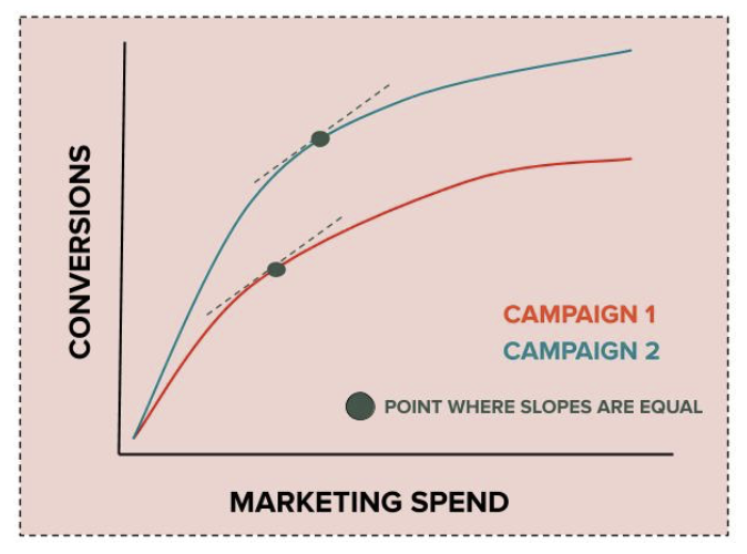
Campaign-level optimization to enable automated bidding
To enable automated bidding so that campaigns do not need to be managed by our marketing team, we need to generate campaign-level spend targets. We can use the same approach that we used to generate channel-level spend targets, above. However, there are some challenges with this approach. For some channels like search engine marketing, we have thousands of campaigns that spend a small amount of money every week. This makes the weekly attribution data noisy. Some weeks these campaigns don’t spend at all, which makes the data sparse. Using this data as-is will result in unreliable cost curves and in turn suboptimal (potentially wildly so) allocation. For other types of campaigns, the data can be clustered in a narrow band of spend. For example, some larger campaigns spend only high amounts and lack historical data in the low spend range. Clustered data such as this makes the cost curve unreliable and highly sensitive to small variations in the input. If the cost curves are unreliable and unstable, the spend allocation generated based on the cost curves will be sub-optimal and unstable. Figure 4 below shows some visual examples of these situations.
Using machine learning to construct better cost curves
Our high-level idea is to train an ML model to predict the expected number of conversions for any campaign, at any spend level. The ML model generates synthetic data, augmenting our real data. Then we fit cost curves to the combined synthetic and real data. The ML model is trained on data from all campaigns so it can learn to identify campaigns that are similar to each other. By doing so, it can learn to fill in the gaps in one campaign’s data by extrapolating from other similar campaigns. To identify similar campaigns, we train it with metadata about the campaigns as features. We use metadata such as the campaigns’ targeting, format, creative size, bidding type, region, and device type.
ML architecture: one ML model per channel
Our channels vary in their need for synthetic data, number of campaigns, campaign sizes, and similarity to other channels. Therefore, we have to train one ML model per channel. Each model is trained on the same training set containing data from all channels. However, we use a different validation set to tune the hyperparameters for each channel’s model. The validation set for a channel consists of recent data for each campaign in that channel, since we care more about recent performance. Some ads can benefit more than others from learning about different channels. We account for this at the channel level: each channel’s model has a set of weights Wc, one per channel. We include these weights in the model’s loss function and tune them as hyperparameters during training. For any channel, if it benefits from learning from a channel c, then Wc takes on a high value. This allows each channel’s model to select the degree to which it uses data from other channels. To tune hyperparameters, we use sequential hyperparameter optimization with scikit-optimize.
Choosing the right amount of ML-generated data
When generating synthetic data, there is a tradeoff to consider. If we generate too much of it, the signal from the real data gets drowned out. If we generate too little, our cost curves aren’t accurate. There is a sweet spot for how many synthetic data points to generate. This sweet spot varies by campaign. Some campaigns have enough accurate real data and need little or no synthetic data, while others need much more. To find this sweet spot for a campaign, we try a range of different values. For each value, we generate that many synthetic data points, fit the cost curve, and evaluate the accuracy of the curve on the validation set. Then, we can simply do a grid search and pick the value that produces the most accurate cost curve. We need to run this grid search for thousands of campaigns. Since each process is independent of the others, we can parallelize them with joblib.Parallel. Running on a Databricks node with hundreds of cores achieves a greater than 100x speedup over no parallelism.Conclusion
Efficient marketing at scale is key to the growth of DoorDash’s top line as well as bottom line. The Marketing Automation platform described above has begun managing some of our marketing team’s weekly budget. As we continue to roll it out to more channels and campaigns, we expect to lower our marketing costs by 10 to 30 percent while reaching the same number of customers. In addition, the platform is also changing the nature of digital marketing at DoorDash. Until now, marketing team members at DoorDash have focused on three things:- Developing marketing strategy,
- Executing it by creating campaigns, and
- Monitoring and managing campaigns to optimize their performance.
- Reacting faster to new data and publishing bids at a cadence closer to real-time
- Extending our approach to operate at the keyword level for search engine marketing
- Switching to an ML-based lifetime value model so that we can optimize our spend for users’ total lifetime value rather than for one-time conversions
- Building a UI layer on top of the platform to allow marketers to fine-tune and monitor performance
- Introducing randomized exploration in the model to sacrifice short term performance in favor of long-term optimization
- Accounting for seasonal changes (from day of week to time of year) and anomalies