Sharpening the Blur: Removing dilution to maximize experiment power

When it comes to reducing variance in experiments, the spotlight often falls on sophisticated methods like CUPED (Controlled Experiments Using Pre-Experiment Data). But sometimes, the simplest solutions are the most powerful and most overlooked – like reducing or eliminating dilution. This unglamorous yet effective technique is free, easy to implement, and plays nicely with other variance reduction methods.

So what is dilution? Dilution happens when we track users in an experiment who could not possibly have been impacted by the treatment. To illustrate, imagine you’re testing a feature to improve conversion on the checkout page of your company’s website. You’d like to test the hypothesis that changing the web checkout button from blue (control group) to green (treatment group) will improve your conversion rate. You’ll randomly assign users to control and treatment groups using a hash function keyed on their user_id’s.

Your product manager asks whether we can increase the power of your experiment by also randomly assigning non-affected users who visit the app into the experiment’s treatment and control groups. You won’t actually change the checkout button’s color in the app – only the website. Nevertheless, you could assign app visitors to treatment and control using the same hash function and increase the experiment’s sample size.

Will simply assigning app users to control and treatment groups increase the experiment’s power, even though we are not making any changes to the app? Of course not! In fact, as we’ll show in the next section, it will reduce the power of the experiment. Despite the fact that including ineligible populations is harmful to experimental measurements, this is a common mistake made throughout the tech industry (as noted in Kohavi et al. and Deng et al.)

Numerical Example

Continuing the example from above, suppose we are changing the checkout button color on a web page, but otherwise making no change to our apps. Let’s say that 70% of users who land on the checkout page will convert to placing an order. The conversion can be represented by a Bernoulli random variable with 𝑝=0.7 and standard deviation:

Van Bell et al (2008) showed that for a metric with standard deviation and collected sample size n, the minimum detectable effect Δ we can measure with a confidence level of 95% and a power of 80% requires a sample size as follows:

If we want to measure a change in signal Δ with a confidence level of 95% and a power of 80%, then the sample size we need is:

Thus to measure a 1% change in checkout conversion rate, we would need a minimum sample size of 𝑛 = 16*0.21/0.01² = 33,600 users to land on our web checkout page.

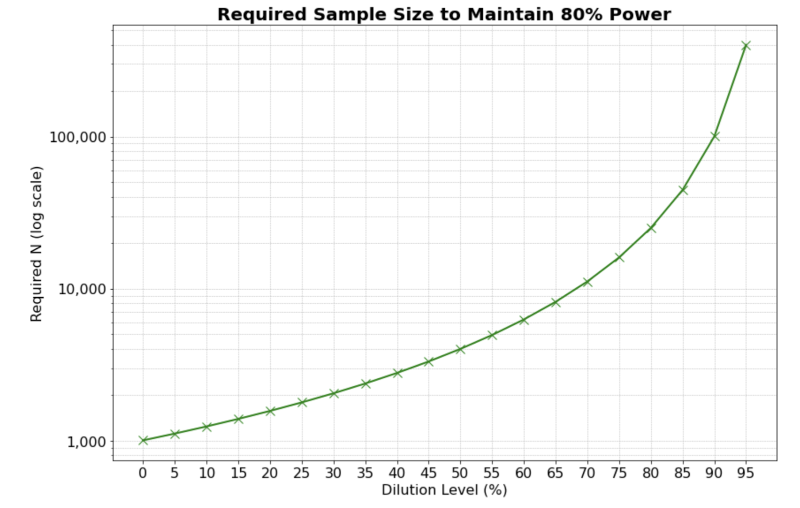
But what if we accidentally include users who land on the app checkout page, which is not impacted by the experiment? For simplicity, let’s say that the app and web checkout pages have equal conversion rates of 70% and equal volumes of users. Let’s define the dilution factor 𝑑 as 𝑛_{𝑑𝑖𝑙𝑢𝑡𝑒𝑑} = 𝑑 * 𝑛_{𝑒𝑙𝑖𝑔𝑖𝑏𝑙𝑒} so 𝑑=2 in this case. As we dilute the experiment, the signal 𝛿 intuitively shrinks as 𝛿_{𝑑𝑖𝑙𝑢𝑡𝑒𝑑} = 𝛿_{𝑒𝑙𝑖𝑔𝑖𝑏𝑙𝑒} /𝑑 while the the minimum detectable effect, or MDE, using the formula above shrinks as 𝛥_{𝑑𝑖𝑙𝑢𝑡𝑒𝑑} = 𝛥_{𝑒𝑙𝑖𝑔𝑖𝑏𝑙𝑒} /√𝑑. Because the signal shrinks faster than the MDE, dilution from app checkout traffic — which is ineligible for the experimental treatment — will spoil our ability to measure a change in eligible web checkout traffic.

Put another way, dilution increases the sample size by a factor of d, but increases the required sample size to maintain MDE by 𝑑². This relationship is plotted in Figure 1 below.

Figure 1: A simulated A/B test showing that dilution has a non-linear impact on experiment sensitivity. Experiments with even 25% dilution will experience a doubling in duration to maintain the same level of power *gist*.

With our accidental dilution from users landing on the app checkout page, that same 1% change in web checkout conversion now corresponds to a 0.5% change in overall web + app conversion because half the conversion happens on the unchanged app. So for the diluted experiment Δ=0.005, we would need 𝑛 = 16*0.21/0.005², 134400, or four times as many users in the overall diluted experiment, which translates to twice as many users needed to land on the web checkout page.

Mistakes that drive dilution

Below are four common mistakes that cause dilution.

Mistake 1: Evaluating everything everywhere all at once

A common cause of experiment dilution is choosing to use too broad of a brush at the outset by evaluating all users at an application’s entry point by encompassing all experiments simultaneously and logging all of those evaluations as real. For example, as shown in Figure 2, an experimenter may create an evaluation class that assigns users to different experiments as soon as they engage with the app without considering whether the changes being tested might affect the user experience. This process may simplify the technical implementation of experiment assignments, but it overlooks the nuanced but critical impact of getting sensitive results. A possible resolution to the problem is shown in Figure 3.

Figure 2: This diluting approach to structuring experiment assignments within a codebase shows all experiments being evaluated and logged as a user enters the application flow. Evaluation results are then used downstream to decide which feature should be shown.

*Figure 3:* This is a corrected, undiluted design that performs and logs experiment evaluation only if a user reaches a particular feature trigger. For instance, if a user reaches the checkout page, we then can decide to show either the control or treatment version of that page.

Mistake 2: Overriding treatment evaluations

This kind of dilution can occur when implemented features are conditional on other user attributes. For example, as shown in Figure 4, the product side might require changing the color of a “purchase” button at the end of a checkout page from blue (control) to green (treatment) only on the web, leaving the mobile checkout experience unchanged.

Figure 4: This example highlights a case where the treatment assignment evaluation is being overwritten by downstream business logic. In this example, dilution is created by including non-web users who fall in the control group.

Dilution occurs if mobile checkouts are included in experiment exposure events. Mobile users see no difference between control and treatment, so they can’t possibly contribute to the experiment’s signal, or mean treatment effect. They do, however, dilute the signal. Figure 5 shows a possible correct implementation.

Figure 5: This is a corrected implementation, where evaluation is done only where the feature change is implemented. Internally, our platform supports user segments, so we can perform the evaluation while smartly taking into account a variety of user attributes (e.g, app-version, region, platform)

Mistake 3: Not managing unintentional traffic

Another potential pitfall in experimental design revolves around the inadvertent inclusion of unintentional traffic in a service's usage data. This traffic typically falls into three categories: bots, load-testing traffic, and unintentional service integrations. Bots often are filtered out with security measures such as authentication checks; nonetheless, they may still dilute experimental results that rely on identifiers like device IDs, where no user login is required. Similarly, load testing can be managed by ensuring traffic is not logged or purging it downstream.

The biggest challenge is how to handle traffic requests from unintentional service integration. One example might be a feed service that provides an API for retrieving a user's favorite restaurants. While this service normally is accessed by the mobile app's backend-for-frontend (BFF) after user authentication, which indicates legitimate user activity, it might also be used by a notification service from a different team seeking to craft personalized emails around a user’s favorite restaurants. That service would use user_ids from a much broader segment than those actively engaging with the app. If the feed service fails to distinguish between requests for legitimate user activity and those from the notification service, any experiments involving "GetFavorites" logic may be diluted because of that wider segment capture. Perhaps even more problematic, as shown in Figure 6, is that if the feed service triggers downstream requests to other services, all downstream experiments could be diluted.

Figure 6: In this diagram feed service normally gets requests from authenticated users of the BFF. service. Nonetheless, it also has an integration with the notification service. Unfortunately, requests from notification don’t reflect legitimate user activity, diluting experiments involving both feed service and other downstream services.

Mistake 4: Including all predictions from a Machine Learning test

In machine learning, where experiments often aim to measure impacts from small adjustments to a model, experiments are often highly diluted unless the experimenter takes great care to avoid dilution. Small tweaks to features, slight recalibrations of models, or minor variations in algorithms can lead to performance improvements that, while potentially small individually, can compound to significantly better outcomes. The trouble comes when these subtle changes must be measured through severe dilutions in online tests.

Consider an example of two classification machine learning models that differ by the slimmest of margins. Visually, as represented in Figure 7, the decision boundaries imposed by these models might be very similar, leading to identical outcomes in the vast majority of evaluations. If the two models make the same prediction for a given point, then including that prediction in the experiment analysis dilutes the signal. Only the points where the two models make different predictions can contribute effectively to the signal. In such a high-dilution scenario, the diluted treatment effect may be so small that a poorly designed online test to detect performance differences ultimately will fail.

Figure 7: In this figure, two ML models make similar predictions, and only a few data points have different predictions. If an experimenter ran an online A/B test that included all predictions, no difference would be detected. *Image source*

Although dilution is most obvious in the case of classification models, experiments based on other model types often suffer from dilution as well. For example: an A/B test of different versions of a ranking model would suffer from dilution for any query where the two models produced the same ranked list (or when the user never viewed any differing items in the ranking). An experiment testing two different regression models could also be diluted if, for instance, we round the prediction before showing it to the end user, as we often do for models that predict the delivery duration. It’s up to the experimenter to determine the extent to which dilution will spoil the results of an experiment.

Resolving dilution

There are two ways to solve for known sources of dilution: 1) real-time adjustment or 2) post-processing adjustment.

Real-time adjustment

To prevent dilution from happening in the first place, we recommend placing your experiment exposure event — its triggering event — as late as possible in the code. This helps ensure that events are generated only for users who are eligible to see them. This best practice offers a few advantages:

Accuracy: It precisely captures the subset of users who are genuinely affected by the treatment change.
Clarity: It results in a clean dataset for analysis, which can reduce manual effort at the experiment analysis stage.
Efficiency and reliability: Because the code only evaluates one or a very small set of experiments, exposure logging footprints and time spent evaluating experiments can be reduced considerably. Within some codebases, DoorDash runs hundreds of concurrent experiments; evaluating too much at once can impact both latency and app crash rates.

While generally positive, real-time adjustment should be done with a few important considerations in mind:

Planning: Perform sufficient planning and QA at the start to ensure that the triggering event is incorporated correctly before the experiment begins.
Flexibility: Real-time adjustment may not always be feasible because of technical limitations. For example, it may be too costly or complex to evaluate counterfactual predictions from an ML model in real time or to evaluate multiple code paths in order to know which experiences are different.

Post-processing adjustment

In post-processing, we retroactively differentiate between impacted and non-impacted user interactions to apply filters on the exposures or metrics datasets. Post-processing provides a couple of advantages:

Salvaging data: Post-processing can correct exposure events after the fact that were placed poorly in the codebase. This can save experiments that might otherwise have had to be re-run.
Adaptable: Post-processing can manage complex systems in which real-time adjustments are impossible. For example, there may be a separate evaluation pipeline to compute counterfactual predictions from ML models that are used purely for post-processing filtering.

You should balance those advantages, however, against some cautionary considerations:

Log accuracy: Ensure that user-interaction logs are absolutely correct, because post-processing relies on that accuracy.
Analysis complexity: Post-processing can add a layer of complexity to data analysis because it requires more sophisticated data processing techniques. In ML applications, for example, balanced experiments require evaluating both models for both groups. To use post-filtering in this case, be certain that the synchronous model does not impact the asynchronous model in any way; for instance, features must be taken from the same moment in time for both models. In practice, this can be a greater effort to implement.

Handling dilution from unintended traffic

The two approaches above can help reduce known sources of dilution, but can’t protect a system from unintentional dilution. As we’ve mentioned, a service may be called by bots or by other internal services masquerading as real users. To manage this kind of dilution, two solutions can be implemented:

Distributed tracing: This technique tracks requests as they flow through various services and components of a distributed system and can be highly effective in identifying sources of non-real user traffic. Distributed tracing starts the moment a user interacts with an application; as the request flows through the system, the trace is tagged with a variety of metadata, for example, which upstream services were involved in the request. Usually, traces are used to understand traffic patterns and performance bottlenecks. But in the realm of experimentation, distributed tracing also serves as a reliable way to identify and filter traffic that should not be evaluated as part of experiments. For example, distributed tracing could prevent the logging of experiment evaluations that don’t originate from the BFF layer.
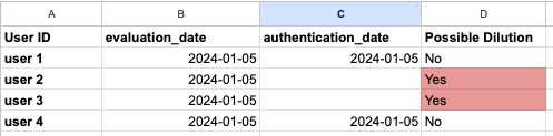
Authentication logs: A somewhat less ideal solution for managing unintentional dilution is to perform post-filtering of experiment evaluations based on authentication logs. For example, if there is a user present in an experiment’s evaluation logs that shows no trigger of an authentication event — in other words, no login or app visit — that’s a good indication that the user is an invalid entry triggered by interacting services, as shown in Figure 8.

Figure 8: In this example, users 2 and 3 have experiment evaluation logs but don’t exist in the authentication logs, indicating that they were created through an invalid path and are not real users visiting the app.

Filtering users based on authentication logs is less than ideal for a couple of reasons:

This method can’t reliably remove all sources of dilution. A user might have an authentication log but still be generating dilution because they don’t interact with the experimental feature.
Analysis becomes more complex because you must perform checks against real app user visits.

In the absence of better logging through tracing, however, this filtering approach is still valuable to detect unknown sources of dilution and salvage experiments with severely degraded sensitivity.

Real-world examples of dilution at DoorDash

Example 1: Fraud targeting model

As with most online businesses, DoorDash uses a model to score the probability that any given checkout is being made by a fraudster using a stolen credit card. If the probability exceeds a given threshold, we require additional verification from the user before completing checkout — for example, scanning an image of the physical credit card. When we release a new version of the checkout risk model, we tend to A/B test it against the incumbent model to make sure we get the expected reduction in fraud costs. If a user is in the control group, the incumbent model decides whether or not the transaction gets step-up verification; if the user is assigned to the treatment group, then the challenger model makes the decision.

Scoring two risk models synchronously before allowing the user to checkout would add too much latency to our system. Therefore, each user is assigned either to control or treatment first. After that, one model is scored synchronously while the other begins scoring asynchronously. Our risk checkout system is designed to handle this common use pattern, so we can guarantee that the features sent to the models will be identical whether they are scored synchronously or asynchronously.

As a result, our experiment is very diluted – all users receive an experiment assignment event at checkout, regardless of whether either model would have applied friction. Each model only applies step-up verification to a tiny fraction of checkouts, generating extreme dilution, as shown in Figure 9.

Figure 9: Ideally, we want our experiment to include the regions labeled 3, 4, 7, and 8. We can exclude regions 1 and 2 because neither model selected those users for step-up verification. We can also exclude regions 5 and 6 because both models selected thodase users, meaning there can be no possible treatment effect.

Here are some real numbers that show how powerful this technique is:

The diluted experiment, which tracked all users eligible for step-up verification over the experiment period, tracked a total of 44.5 million users. The experiment readout of our primary fraud cost metric showed a reduction of -0.9677% [-8.4302%, +6.4948%], which was nowhere near statistical significance (t = 0.25, p value = 0.799). But the post-filtered experiment included only 292,000 users and showed a statistically significant reduction of our fraud cost metric over the experiment’s time period — -9.74% [-15.7402%, -3.7397%] (t=3.18, p value = 0.001465). Removing the dilution allowed us to increase sensitivity by a factor of (3.18/0.25)^2 = 160!

Note that the metric needs to be carefully re-scaled to represent the total global impact. We can do this easily, however, using the absolute changes in metric values (not shown) multiplied by the number of users included in the undiluted analysis.

Example 2: Supply-demand rebalancing

DoorDash’s Supply-Demand team aims to build levers to manage existing and future supply-demand imbalances. Historically, most regions managed by the team had good supply, so we found fewer and fewer instances where the system had to intervene. While this was a positive outcome from a product standpoint, it challenged the team in its effort to develop and evaluate new measures designed to act during supply shortages. As our systems kept improving, there were fewer and fewer opportunities for how we could validate our ideas.

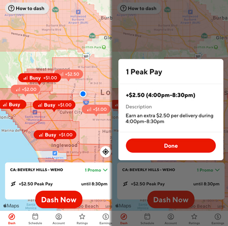
Fortunately, our experimental design benefited from advanced knowledge about the application of specific levers, allowing us to distinguish between the user experiences in treated versus untreated region-time segments. For example, in one test we wanted to check if we should just adjust the timing of the peak pay incentives Dashers get. Our hypothesis was that we should offset the incentive timing by 30m, to allow Dashers more time to get mobilized and get on the road. Given that this lever was only deployed in less than 15% of regions, by removing the regions that could not possibly be impacted by our treatment intervention, we were able to improve the sensitivity of our metrics by 10x to 15x.

Figure 10: Heatmap screen on the Dasher app that lets Dashers know about existing and future incentives. This lever is rarely deployed; removing dilution from untreated regions allowed us to increase sensitivity 10 to 15 times.

Conclusion

In closing, dilution poses a substantial threat to the integrity and effectiveness of running experiments. Through real-world examples and empirical evidence from within DoorDash, we’ve witnessed firsthand the detrimental consequence of neglecting to address dilution. Thankfully, we can remove dilution from experiments by either real-time or post-processing adjustments to recover the power of experimental measurements.