
For DoorDash, being able to predict long-tail events related to delivery times is critical to ensuring consumers’ orders arrive when expected. Long-tail events are rare instances where time predictions are far off from actual times and these events tend to be costly. While we previously improved long-tail predictions (as explained in this previous post) by tweaking our loss function and adding real-time signals, we wanted to improve the predictions further by using a gamma distribution-based inverse sample weighting approach to give long-tail events more weight during model training. In this post, we will go into detail about how we used gamma distribution to improve model performance.
Significance of accurate long-tail predictions
Before we dive deeper, let’s quickly recap why the accuracy of DoorDash’s delivery estimates (ETAs) is so important. ETA (estimated time of arrival) is a promise to the consumer of the time when the order will arrive at their door. Under-prediction results in a really bad ordering experience (a late delivery) and over-prediction (giving a higher estimate) might result in consumers not placing an order or getting a delivery before they get home to receive it. Moreover, delivery times are difficult to predict, particularly because of the wide variability in order preparation times, road traffic conditions, availability of Dashers (delivery drivers), and time to find parking and navigate to residential addresses. The unpredictability of these components leads to costly long-tail events. To improve these estimates, it is important to model the distribution and tweak the loss function to better penalize long-tail events (both early predictions and late predictions).
Finding the best distribution to model delivery times
In our previous post, we explained that we can tweak the loss function and add real-time signals to our machine learning (ML) model to improve accuracy. To iterate and improve on those tweaks, we wanted to employ the loss function that replicates our delivery time distribution as accurately as possible.
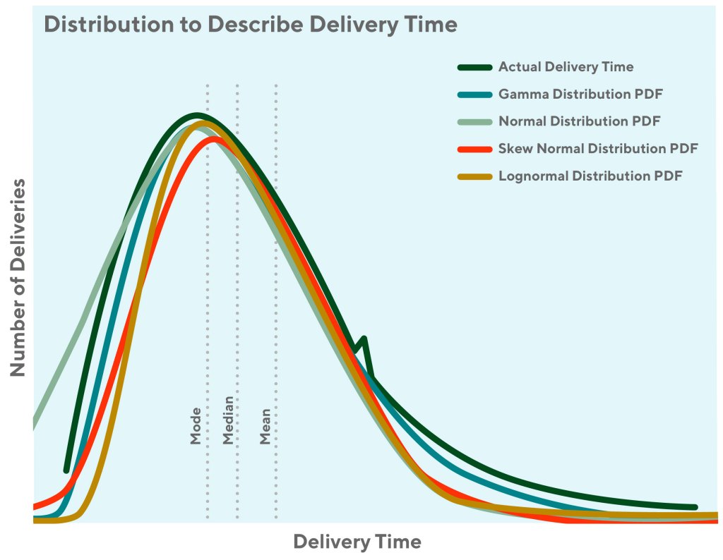
We explored a few distributions before finding the best fit as shown in Figure 1. Let’s actually start with a brief review of the commonly used distributions:
- Normal distributions are commonly used in the natural and social sciences to represent real-valued random variables whose distributions are unknown, because they are symmetrical, mathematically easy, and fit a wide collection of events. You might know this distribution from the very fundamental central limit theorem.
- Log-normal distributions are used to model phenomena with fatter right tails and which take on only positive values (no left tail). For example, in highly communicable epidemics, such as SARS in 2003, the number of hospitalized cases is a log-normal distribution. In economics, the income of 97%–99% of the population is distributed log-normally.
- Gamma distributions are used to model phenomena with a long tail on the right side. For example, the sizes of the insurance claims follow a Gamma distribution, so does the amount of rainfall accumulated in a given time period.
To quantify the similarity of each distribution with our empirical target distribution, we used the Kolmogorov-Smirnov test (K-S test). The statistics of K-S test results can be used to indicate the similarity between two given distributions. It ranges from zero to one, where zero means totally different and one means exactly the same. Typically, K-S test statistic output <0.05 is used to reject the hypothesis that the two given distributions are the same. From the K-S test result in Table 1, we found both log-normal and gamma almost perfectly fit our empirical distribution. In practice, these two distributions are often used to model the same phenomena. For our use case, we decided to go for the gamma distribution to model delivery estimates. In the following section, we explain the fundamental characteristics of the gamma distribution and why they suit the problem we are trying to solve.
| Distribution name | K-S test statistics |
| Normal | 0.512 |
| Skew normal (asymmetric) | 0.784 |
| Log-normal | 0.999 |
| Gamma | 0.999 |
Stay Informed with Weekly Updates
Subscribe to our Engineering blog to get regular updates on all the coolest projects our team is working on
Please enter a valid email address.
Thank you for Subscribing!
What is the gamma distribution?
Gamma distributions have been used to model continuous variables that are always positive and have skewed distributions. It is often used to describe the time between independent events that have consistent average time intervals between them, such as rainfalls, insurance claims, wait time, etc. In oncology, the age distribution of cancer incidence often follows the gamma distribution, whereas the shape and rate parameters predict, respectively, the number of driver events and the time interval between them. In transportation and service industries, the gamma distribution is typically used to estimate the wait time and service time.
The gamma distribution function has two parameters: a shape parameter and a rate parameter (Figure 2). The shape parameter α represents the number of independent events we are modeling. When the shape parameter (α) is equal to one, the gamma distribution becomes an exponential distribution. Thus, the gamma distribution is essentially the summation of several exponential distributions. In our case, the shape parameter (α)is equal to four gives the best fit to the actual delivery time distribution curve. Since the delivery time is determined by numerous factors, α value does not necessarily indicate there are four independent events. It may imply the underlying events that drive the shape of the gamma distribution are equivalent to four independent events. When keeping everything else constant, increasing causes the peak of the probability density function (PDF) curve to move to the right side.
The rate parameter β represents the average time between these events. If we keep everything else the same, reducing the rate parameter (which means increasing the scale parameter) will cause it to take longer to observe the same number of events, thus, a flatter PDF curve.

The PDF for gamma distribution is given by equation (1).

Now that we understand the gamma distribution, the question arises about how we can use the gamma distribution to model sample weights in our training process.
Using gamma distribution to make better predictions
To make better predictions on the low-frequency long-tail events, we want to allow the model to learn more information from these events. This can be achieved by assigning more weight to these events during the model training process. We use a weight function to assign the weight to different data points. These were the steps we followed:
- First, we find the best-fit gamma distribution for the delivery duration data. In our case, we found α=4 and β =1 to have the best fit.
- Next, we set the weight function inversely proportional to the PDF of the gamma distribution to allow the model to learn from the rare long-tail events.
- We split the training data samples into two groups at the peak density (the Mode). The group on the left side of the peak density has a shorter delivery time, and the right side group has a longer delivery time.
- The sample weights of the data points are tuned differently for samples on the left and right sides of the peak according to business constraints. This helps tune for earliness as well as lateness.
Through this process, we reduced 20-minute lateness by 11% (relative). Particularly, the super long-tail parts were better predicted (Figure 3). The gamma weight trained model doubles the number of long-tail predictions than the Asymmetric Mean Squared Error (AMSE) method. On top of the great results we saw, certain characteristics of gamma distribution enabled us to effectively tune our loss function to incorporate desired business outcomes.

Advantages of customizing gamma distribution
To achieve better business results, the model needs to make accurate predictions on the right long-tail events and make sure we are not over-predicting faster deliveries. The nature of gamma distributions helped us to accomplish both goals, allowing for wider distribution of prediction results and better coverage on earliness and long tail:
- Earliness and lateness were better balanced by adjusting the weight according to business impact.
- AMSE distribution does help capture earliness and lateness nuances, but clearly, gamma distribution gives a much longer-tail coverage as you can see in the plot.
- That said, there are some shortcomings of this methodology:
- We need to tune an extra set of weights (left/right) during retraining each time.
- In scenarios when you have continuous retraining through automated pipelines, keeping a constant set of left and right weights can cause degradations in model performance if these weights are not regularly fine-tuned as per the data.
Conclusion
We improved the prediction performance on long-tail events by tweaking the loss function with a customized sample weighting approach based on the gamma distribution. The AMSE is an asymmetric loss function designed to model a right-skewed distribution. It captures the long-tail events that follow a skewed quadratic distribution. However, the gamma-based weight function distribution is more similar to the actual distribution of delivery durations and has more advantages compared to AMSE:
- Compared to the AMSE loss function, it decays slower on the long-tail part.
- Separating the weight function at the mode of the distribution gives us more flexibility to tune both earliness and lateness.
We have not stopped here, and we will continue exploring new options to improve the accuracy of our estimates. If you are passionate about building ML applications that impact the lives of millions of merchants, Dashers, and customers in a positive way, consider joining our team.