

Making accurate predictions when historical information isn’t fully observable is a central problem in delivery logistics. At DoorDash, we face this problem in the matching between delivery drivers on our platform, who we call Dashers, and orders in real time.
The core feature of our logistics platform is to match Dashers and orders as efficiently as possible. If our estimate for how long it will take the food in an order to be cooked and prepared for delivery (prep time) is too long, our consumers will have a poor experience and may cancel their orders before they are delivered. If prep time estimates are too short, Dashers will have to wait at merchants for the food to be prepared. Either scenario where we inaccurately estimate food prep time results in a poor user experience for both the Dashers and the consumers. Noisy estimates will also affect the network by reducing the number of available Dashers who could be on other orders but are stuck waiting on merchants.
At the heart of this matching problem is our estimation of prep time, which predicts how long it takes for a merchant to complete an order. The estimation of prep times is a challenge because some of our data is censored and our censorship labels are not always reliable. To manage this, we need an accurate but transparent modeling solution for censorship that is not readily available in the machine learning toolbox.
We tested methods ranging from Cox proportional hazard models to neural networks using custom objective functions with little success. Our winning solution was a simpler pre-adjustment to our data that allowed us to use common gradient boosting machines (GBMs). In this article, we will define the problem in greater depth, walk through these ideas we tried, and explain the technique we developed that satisfied our constraints.
The prep time estimation challenge: dealing with censored data
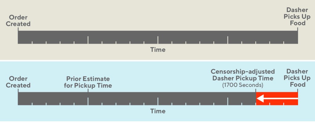
To understand the challenges of estimating prep time let's first take a look at the ordering process, which can be seen in Figure 1, below:

After an order is sent to the merchant, the Dasher is assigned to the order and can travel to the merchant at the estimated prep time, but may end up waiting until the order is ready. If the Dasher waits at the store for more than a couple of minutes, we have some confidence that the order was completed after the Dasher arrived. In this case, we believe the observed food prep time to be uncensored. This data is high quality and can be trusted. Alternatively, had the Dasher not waited at all, we believe the prep time data to have been censored, since we don’t know how long the order took to be completed.
The data here is unique for two reasons. Much of the data is left censored - meaning that the event occurs before our observation begins. In typical censorship problems, the timing is reversed. It is also noisily censored, meaning that our censorship labels are not always accurate.
Herein lies our challenge. We need to build a prediction that is accurate, transparent, and improves our business metrics. The transparency of our solution will allow us to learn from the censorship that is occurring and pass feedback to other internal teams.
With these requirements, we’ll describe methods that we tried in order to create a model that could handle censorship for our estimated prep times. Finally we’ll go into depth on the solution which finally worked for our use case.
The first three prep time estimation solutions we tested
We had competing priorities for a winning solution to the prep time problem. Our production model needed to incorporate the concept of censorship in an interpretable and accurate way.
Our initial approach was to discard the data we thought to be censored. This approach did not work because it would bias our dataset, since removing all the censored data would make our sample not representative of reality. Important cases where dashers were arriving after food completion were being completely ignored. In terms of our criteria, this naive approach did have an interpretable censorship treatment, but failed in terms of accuracy, since it's biased.
We tested a few iterations of Cox proportional hazard models. These have a very transparent treatment of censored data but can be inaccurate and difficult to maintain. Offline performance was poor enough to convince us that it was not worth spending experimental bandwidth to test.
We then tried more sophisticated black box approaches that incorporated analogous likelihood methods to Cox models, such as XGBoost’s accelerated failure time loss functions and adaptations of WTTE-RNN models. These solutions are elegant because they can handle censorship and model fitting in a single stage. The hope was they could also provide a similar degree of accuracy to censorship problems that ordinary GBMs and neural networks can provide to traditional regression problems.
For both of these black box approaches, we found that we were unable to get the offline metrics that were necessary to move forward. In terms of our constraints, they also have the least interpretable treatment of censored data.
A winning multi-stage solution
The final technique we tried involved breaking the problem up into two stages: censorship adjustment and model fitting. An ideal model will make the most of our censored data, incorporating prior estimates of food prep time. We incorporate prior estimates by adjusting the data, and then fit a model on the adjusted data set as if it were a traditional regression problem.
If a record is censored and its prior estimate is well before a Dasher’s pickup time, then our best estimate for that data point is that it occurred much earlier than observed. If a record is censored and our prior estimate is near or after a Dasher’s pickup time, then our best estimate is that it occurred only slightly before we observed. If a record is uncensored, then no adjustment is necessary.
By comparing the observed timing to the prior expected timing, we create an intermediate step of censorship severity. Identifying and adjusting for censorship severity is the first stage in our two-stage solution, effectively de-censoring the data set. The second stage is to fit a regression on the adjusted dataset.
The two-stage approach carried just the right balance of transparency and model accuracy. It let us deploy boosting techniques leading to greater accuracy. This approach also let us inspect our data directly before and after adjustment so that we could understand the impacts and pass learnings along to partners in the company.
Not surprisingly, this method also led to the biggest metrics improvements, improving our delivery speeds by a statistically and economically significant margin.
| Transparency of censorship treatment | Improvement of accuracy and business metrics | |
| Drop uncensored records | High | Low |
| Proportional hazard models | Medium | Low |
| XGBoost AFT | Low | Low |
| WTTE-RNN | Medium | Medium |
| Two-stage adjustment | High | High |
Figure 2, below, shows the delivery times observed in a switchback test, comparing the two-staged and incumbent model at different levels of supply.

A recipe for building a censorship adjustment model
Below is a brief recipe to handle censorship in a model. There are three example data points: one is completely uncensored, and the other two are censored to different degrees. We select a simple censorship adjustment method here, a linear function of the censorship severity.
| Record # | Target Value (Directly observed) | Is Censored (Directly observed) | Prior Estimate (built from baseline model) | Censorship Severity = Observed Arrival Time - Prior Estimate | Adjustment = 0.2 * Severity | Adjusted Target (Used as modeling target) |
| 1 | 1500s | No | 2000s | NA | 0s | 1500s |
| 2 | 1750s | Yes | 1600s | 150s | 30s | 1720s |
| 3 | 2000s | Yes | 500s | 1500s | 300s | 1700s |
Note that our uncensored data is not adjusted in any way. Transparency allows us to check if this was desirable or not, enabling iteration on our censorship scheme.
Figure 3, below, illustrates the adjustments that were made. In the uncensored case, our model targets the time at which the Dasher picks up food. In the censored case, our model targets an adjusted variant of that data.
The earlier our preliminary naive estimate is, the larger the adjustment will be. Since the ground truth is unobservable in censored situations, we are doing the next best thing, which is to inform our data with a prior estimate of the ground truth.
The censorship adjustment introduces a need for other hyperparameters. In the example above, we use a constant value, 0.2. The larger this scale parameter is, the greater our adjustment will be on censored data.
Conclusion
It’s important to identify key properties of a modeling solution. Many times, there are elegant options that seem appealing but ultimately fail. In this case, the two-stage adjustment is a clever elementary adjustment. Complex likelihood methods were not necessary. By adding a two-stage adjustment, we achieved our goals of accuracy and transparency that wasn’t available from off-the-shelf solutions we tried initially. The result is that a simple solution gave us the accuracy and transparency that we were seeking.
Censored data is a common problem across the industry. As practitioners, we need to work with the data that’s available regardless of how it’s obtained. Sometimes, experimental design leads to subjects who drop in and out. Other times, physical sensors are faulty and fail before the end of a run. This two-stage adjustment is applicable to other censored problems, especially when there’s a need to disentangle the challenges from censorship and the underlying modeling problem.
Header photo by Hunter Harritt on Unsplash