
For any operations-intensive business, accurate forecasting is essential but is made more difficult by hard-to-measure factors that can disrupt the normal flow of business. For DoorDash this problem is especially acute as any major deviations from our supply and demand forecasts have the potential to disrupt orders and provide a worse experience for consumers and Dashers. To generate accurate forecasts, we take into account seasonality and multiple factors via modeling and feature engineering. However, there could be factors affecting the orders but the true relationship between the demand and factor requires additional information beyond simple feature engineering. In those cases, we leverage causal inference methods to capture the additional information.
In this post, we first discuss our general strategy when using causal methods to improve forecast accuracy, and then follow with two specific cases from DoorDash. The first case highlights the importance of accounting for macroeconomic factors via causal inference, with an example that focuses on predicting how tax refunds will affect order volume. The second case describes how to disentangle the impact coming from two concurrent factors. To demonstrate the concept, we have included a case study of daylight saving (which overlapped with Halloween in previous years, but not in following years). The application of these causal inference approaches helps us generate more accurate forecasts.
Overview of forecasting at DoorDash
The Forecasting Team at DoorDash established scalable solutions to generate forecasts spanning demand planning, support, finance and now cut across a broad range of operational touchpoints. When generating the forecasts, we leverage time-series methods to get the correct trend and seasonality abstracted from the temporary fluctuations affecting target metrics such as weather and promotions.
The basic approach to account for temporary fluctuations is to define features (e.g., precipitation for weather, one-hot encoding holidays) and incorporate those features in the model. However, some temporary sources of fluctuations (e.g., tax refunds, child tax credits) may not have a direct measure/feature, which makes them hard to detect and account for in our forecast. For these types of factors, we leverage causal methods such as difference-in-differences and preprocess the demand series so that we can calculate the correct trend.
When facing fluctuations that cannot be incorporated using feature engineering, the Forecasting Team uses the following strategy to calculate the impact:
- Identify sub-segments of the market that are differentially impacted by the factor causing fluctuations in the demand
- Select an appropriate causal method (e.g., differences-in-differences, synthetic controls)
- Use the chosen causal method and calculate the impact of the factor
- Remove the calculated impact from the target series so that trend is not affected by the factor
Given that every one of these factors is hard to measure in its own unique way, we have collected a series of case studies that demonstrate the challenge of removing their impact from forecasts - and the effectiveness of our method. We will start with an example that looks into how a macroeconomic factor such as tax return affects our order volume. Then we will look into a case where we disentangle the impact coming from two concurrent factors.
Detecting macroeconomic trends: tax refunds case study
Causal inference is useful to measure the impact of macroeconomic factors in the target series. When dealing with factors creating a large and long-lasting increase/decrease in the target series (i.e, the impact is “clear”), identifying and removing the true impact of the factor generates large gains in the forecast accuracy. Most of the time such factors are associated with macro events that could affect consumers and businesses in any industry, such as shelter-in-place orders during the pandemic, child tax credit payments, supply-chain crises, or Federal Reserves’ interest rate increases.
Failing to account for the changes in such macro factors could lead to poor forecasts and catastrophic failures in business operations. For instance, factors such as government stimulus or supply crises could create a temporary boost in the customer demand (or prices). If those factors are not taken into consideration during the forecasting, the statistical models could assume those temporary fluctuations as permanent trends and generate artificially high forecasts, which may mislead decision-makers and lead to large losses.
One area in which the Forecasting Team uses the causal methods is IRS payments to households, which create a temporary increase lasting a couple of months in the consumer spending and order volume. If this impact is not accounted for, the models will generate artificially high forecasts for the weeks that IRS payments end due to the previous demand spike.
Even though we have data on the amount of tax refunds deposited into the bank accounts through the IRS, we cannot directly use it in our models, as (a) consumer segments may respond differently to tax refunds, and (b) tax refunds are not distributed evenly across those consumer segments both within each tax year and across years, implying that tax refund data could not capture the time-varying response of heterogeneous consumer segments to tax refunds. Therefore, we decided to leverage causal inference to incorporate the information lives outside the tax refund data by following the steps outlined below:
- We observed that the consumers' responses located in different zip codes are disproportionate, which is consistent with the Census Pulse Survey showing the heterogeneous relationship between the share of food spending and household income.
- After making the above observation, we decided to use the difference-in-differences method, in which we set the treatment group as the affected zip codes and the control group as the non-affected zip codes .
- We use the following regression to calculate the impact of the tax refunds on the affected zip codes:

where yit is the number of orders in zip code i at date t. δk are the event-date dummies that capture the time-varying impact of the tax refund as the difference between the treatment and control group starting from the first day (i.e., t=0) that large amounts of tax refunds hit the bank accounts. Figure 1 shows the estimated coefficients for the treated zip codes. As expected, the growth in the treated zip codes is higher after receiving the tax returns.

- After calculating the impact for the treated zip codes, we calculate the tax refund impact for each submarket using the share of orders coming from treated zip codes in that submarket.
- We remove the impact from tax refunds in the preprocessing step, and then generate forecasts using the time-series models for submarkets in the United States. Next, we apply post-processing to incorporate the future tax refund impact based on the tax refund phase out in the earlier years.
Table 1 shows the relative improvement in 6-week-ahead forecasts measured in terms of mean absolute percentage error (MAPE) and mean percentage error (MPE) with respect to the baseline forecast (making no adjustment for the tax refunds). Specifically, the relative MAPE/MPE is calculated as:

The results show that preprocessing the tax-refund impact provides a sizable improvement in the out-of-sample performance of the forecast (implying a sizable reduction in the Dx acquisition costs).

The above case is a great example of how we use causal methods to capture the impact of a macroeconomic factor (i.e. the tax refund), creating a large increase in the order volume. Historically, we followed a similar strategy to account for lockdowns during the pandemic. Moreover, we are actively monitoring potential shifts in the macro conditions that could impact consumer demand and brainstorming on causal methods to measure the impact.
Disentangling concurrent factors: daylight saving case study
Causal inference is useful if we have multiple factors affecting the series concurrently and we aim to disambiguate the impact by measuring the contribution of each factor separately. In the presence of concurrent factors, simply putting dummy variables (i.e., one-hot encoding) for those events will not work (because of the multicollinearity problem). Disentangling the impact is helpful to generate more accurate forecasts (especially if those factors occur in different time periods in the future), and to have a clear understanding of the factors driving the target series (among factors other than the concurrent factors).
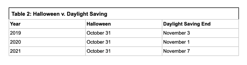
The Forecasting Team leveraged causal methods to measure the impact of the end of daylight saving time in November, which is concurrent with Halloween in the earlier years. Specifically, our team observed that there is a strong increase in the order volume in the week following Halloween and associated the strength with Halloween which coincided with the end of daylight saving in 2019 and 2020 (Table 2). Contrary to earlier years, in November 2021, we observed a strength one week after Halloween. After discussions with business partners, we concluded that one potential factor contributing to a rise in demand is the end of daylight saving. The sun sets an hour earlier, potentially making customers go home earlier rather than eat outside.
To test whether the impact comes from daylight saving, we develop a creative method that leverages the borders between time zones, which is similar to a paper investigating the impact of sunrise on school performance. More specifically, consider Indianapolis and Chicago where Indianapolis is in the Eastern Time Zone (ETZ) and Chicago is in the Central Time Zone (CTZ). Table 3 shows the sunset times before and after the daylight saving time in November 2021 in those two cities. As Chicago gets dark around 4:37 PM (as opposed to Indianapolis getting dark at 5:36 PM), we hypothesize that Chicago locals are more likely to get home right after finishing the day and order food from DoorDash instead of spending time outside in the dark.

To calculate the impact, we identified DoorDash submarkets located around the ETZ/CTZ, CTZ/MTZ, and MTZ/PTZ border (see Figure 2). Then, we classified submarkets east of the border as control (e.g., Indianapolis, Detroit, Amarillo) and those west of the border as treatment (e.g., Chicago, Nashville, Denver).

Then we run the following difference-in-differences model to calculate the impact:

where yit is the order volume at submarket i at date t; post is the dummy variable taking value 1 for the dates after daylight saving went effect on November 7, 2021; treatment is the dummy taking value 1 for the states on the west of the time zone border; the controls are day-fixed effects to capture the weekly seasonality.
We estimate the daylight saving impact as a positive number implying that the order volume increases more for the cities located on the west of the time zone border compared to the ones on the east. Note that the estimated impact will be under biased as the control group is also affected positively from the daylight saving, but not as strongly as the treatment group. Moreover, the calculated impact is abstract from Halloween, as Halloween is relevant for both treatment and control markets (which is captured with post dummies in the above regression). We are planning to use the calculated value when generating forecasts for the daylight saving end on November 6, 2022.
Daylight saving is a perfect case that illustrates how a concurrent factor could affect the consumer demand and remain unnoticed. Such cases require close scrutiny and collaboration with the business partners in addition to discovering creative causal methods to measure the actual impact.
Conclusion
Causal methods are frequently used for estimation (e.g., measuring the impact of promotions) but not for prediction and forecasting. As the forecasting team at DoorDash, we improved the forecasting accuracy of our time-series models by using a creative way of applying causal methods in situations for which we do not have a direct measure of factors driving the demand. Specifically, we discussed use cases of tax refunds and daylight saving in this blog post. As the forecasting team, we are constantly developing and adopting solutions to understand all factors impacting our forecasts, and to generate more accurate forecasts.
Acknowledgements
Many thanks to Kurt Smith, Lauren Savage, Gonzalo Garica, Matt Heitz, Lambie Lanman, Chris Li, and Ryan Schork for sharing their insights on the development, and support on the execution of the ideas in this blog post. Many thanks to Ezra Berger for continuous support, review, and editing on this article.