Building a Gigascale ML Feature Store with Redis, Binary Serialization, String Hashing, and Compression

When a company with millions of consumers such as DoorDash builds machine learning (ML) models, the amount of feature data can grow to billions of records with millions actively retrieved during model inference under low latency constraints. These challenges warrant a deeper look into selection and design of a feature store — the system responsible for storing and serving feature data. The decisions made here can prevent overrunning cost budgets, compromising runtime performance during model inference, and curbing model deployment velocity.

Features are the input variables fed to an ML model for inference. A feature store, simply put, is a key-value store that makes this feature data available to models in production. At DoorDash, our existing feature store was built on top of Redis, but had a lot of inefficiencies and came close to running out of capacity. We ran a full-fledged benchmark evaluation on five different key-value stores to compare their cost and performance metrics. Our benchmarking results indicated that Redis was the best option, so we decided to optimize our feature storage mechanism, tripling our cost reduction. Additionally, we also saw a 38% decrease in Redis latencies, helping to improve the runtime performance of serving models.

Below, we will explain the challenges posed in the task of operating a large scale feature store. Then, we will review how we were able to quickly identify Redis as the right key-value store for this task. We will then dive into the optimizations we did on Redis to triple its capacity, while also uplifting read performance by choosing a custom serialization scheme around strings, protocol buffers, and Snappy compression algorithm.

Requirements of a gigascale feature store

The challenges of supporting a feature store that needs a large storage capacity and high read/write throughput are similar to the challenges of supporting any high-volume key-value store. Let’s elaborate upon the requirements before we discuss the challenges faced when meeting these requirements specifically with respect to a feature store.

Persistent scalable storage: support billions of records

The number of records in a feature store depends upon the number of entities involved and the number of ML use cases employed on these entities. At DoorDash, our ML practitioners work with millions of entities such as consumers, merchants, and food items. These entities are associated with features and used in many dozens of ML use cases such as store ranking and cart item recommendations. Even though there is an overlap in features used across these use cases, the total number of feature-value pairs exceeds billions.

Additionally, since feature data is used in model serving, it needs to be backed up to disk to enable recovery in the event of a storage system failure.

High read throughput: serve millions of feature lookups per second

A hit rate of millions of requests per second is a staggering requirement for any data storage system. The request rates on a feature store are directly driven by the number of predictions served by the corresponding system. At DoorDash, one of our high volume use cases, store ranking, makes more than one million predictions per second and uses dozens of features per prediction. Thus, our feature store needs to support tens of millions of reads per second.

Fast batch writes: enable full data refresh in a nightly run

Features need to be periodically refreshed to make use of the latest real world data. These writes can typically be done in batches to exploit batch write optimizations of a key-value store. At DoorDash, almost all of the features get updated every day, while real time features, such as “average delivery time for orders from a store in the past 20 minutes”, get updated uniformly throughout the day.

Stay Informed with Weekly Updates

Subscribe to our Engineering blog to get regular updates on all the coolest projects our team is working on

Please enter a valid email address.

Thank you for Subscribing!

Specific design challenges in building a feature store

When designing a feature store to meet the scale expectations described above, we have to deal with complexities that are specific to a feature store. These complexities involve issues such as supporting batch random reads, storing multiple kinds of data types, and enabling low-latency serving.

Batch random reads per request add to read complexity

Feature stores need to offer batch lookup operations because a single prediction needs multiple features. All key-value stores support unit lookup operations such as Redis’s GET command. However, batch lookups are not a standard especially when keys are in no particular sequence. For example, Apache Cassandra doesn’t support batch random lookups.

Heterogeneous data types require non-standardized optimizations

Features can either be simple data types such as integers, floats, and strings, or compound types such as vector embeddings or lists. We use integers or strings for categorical features such as order protocol, for whether an order was received by merchants via email, text, or iPad. We use lists for features such as a list of cuisines chosen by a customer in the past 4 weeks. Each one of these data types needs to be individually treated for optimizing storage and performance efficiency.

Low read latency but loose expectations on write latency

A feature store needs to guarantee low-latency reads. Latency on feature stores is a part of model serving, and model serving latencies tend to be in the low milliseconds range. Thus, read latency has to be proportionately lower. Also, typically, writes and updates happen in the background and are much less frequent than reads. For DoorDash, when not doing the batch refresh, writes are only 0.1% of reads. Low-latency requirements on reads and loose expectations with writes gives a direction for building towards a read-heavy key-value store but one that is fast enough for large batch writes.

Identifying the right key-value store by benchmarking key performance metrics 

The choice for an appropriate storage technology helps greatly in increasing the performance and reducing the costs of a feature store. Using Yahoo’s cloud serving benchmark tool, YCSB, we were able to identify Redis as a key-value store option that best fit our needs.

What we need from a benchmarking platform

Before we lay out our benchmarking setup, it is worthwhile to emphasize key requirements of a benchmarking platform. The four major required capabilities of a benchmarking setup are: 

• Data generation using preset distributions

Using data generation is a faster and more robust approach to benchmarking than ingesting real data because it accounts for possible values that a system’s random variables can take and doesn’t require moving data around to seed a target database.

• Ability to simulate characteristic workloads

The workload on a database can be defined by the rate of requests, nature of operations, and proportions of these operations. As long as we can guarantee the same fixed request rate across tests, we can enable a fair comparison between the different databases.

• Fine-grained performance reporting

The suite should be able to capture performance with appropriate statistical measures such as averages, 95th percentile, and 99th percentiles.

• Reproduction of results on demand

Without reproducibility, there is no benchmark, it’s merely a random simulated event. For this reason, any benchmark platform needs to be able to provide a consistent environment where the results can be reproduced when running the same test over and over.

Using YCSB to do a rapid comparison of key-value stores

YCSB is one of the best benchmarking tools out there for analysing key-value stores. So much so that it not only meets all of the needs we described above but also provides sample code to benchmark a vast number of key-value stores. This setup ensures we have a flexible playground for rapid comparisons. Below, we describe our approach of using YCSB to validate our selection of Redis as the best choice for a feature store. We will first describe our experiment setup and then report the results with our analysis.

Experiment setup

When setting up the benchmarking experiment, we need to start with the set of key-value stores that we believe can meet the large scale expectations reliably and have a good industry presence. Also, our experiment design is centered around Docker and aims to optimize the speed of iterations when benchmarking by removing infrastructure setup overheads.

Candidate set of key-value stores

The key-value stores that we experimented on in this article are listed in Table 1, below. Cassandra, CockroachDB, and Redis have a presence in the DoorDash infrastructure, while we selected ScyllaDB and YugabyteDB based on market reports and our team’s prior experience with these databases. The intention was to compare Redis as an in-memory store with other disk-based key-value stores for our requirements.

Database name	Version
Cassandra	3.11.4
CockroachDB	20.1.5
Redis	3.2.10
ScyllaDB	4.1.7
YugabyteDB	2.3.1.0-b15

Data schema

For data storage, we chose following patterns:

• SQL/Cassandra

CREATE TABLE table (key varchar primary key, value varchar)

• Redis

SET key-value
GET key

Input data distribution

For the key-value stores, we set the size of our keys using an average measure on the data in our production system. The size of values were set using a histogram representing size distribution of actual feature values. This histogram was then fed to YCSB using the fieldlengthhistogram property for workloads

Nature of benchmark operations

The benchmark was primarily targeted at these operations

• batch writes
• batch reads
• update

We used the following implementation strategy for batch reads to allow any scope for database-side optimizations across lookups and to minimize network overheads.

• SQL: IN clause 

SELECT value FROM table
WHERE key IN (key1, key2 .. keyM)

• Redis: Pipelining
• Cassandra query language (CQL): Datastax executeAsync

We used the CQL interface for ScyllaDB and the SQL interface for YugabyteDB. 

Benchmarking platform: Docker

We set up our entire benchmark on a 2.4 GHz Intel Core i9 16GB RAM MacOS Catalina 10.15.7 with 8GB RAM and 8 cores available for Docker. The Docker setup for each database had the following:

• Docker containers for DB under test
• Docker container for YCSB
• Docker container for cAdvisor that can track docker cpu/memory

We used Mac as opposed to EC2 instances in AWS to allow rapid preliminary comparisons between the different databases without any infrastructure setup overheads. We used Docker on Mac as it’s easier to get control and visibility on resources in a container-based isolation vs process-based isolation.

As Docker has a measurable effect on performance, we used it with caution and made redundant runs to guarantee the reliability of our results. We validated our Docker setup by comparing improvements reported in local tests with improvements in production using the case of Redis. Check out this study to learn more about the Docker’s impact on benchmarking.

Experiment results

In our experiments, we wrote custom workloads to mix our benchmark operations using two sets of fractions of reads versus writes — one with 100% batch reads and the other with 95% reads. We ran these workloads with 10,000 operations at a time using a batch size of 1,000 lookups per operation. We then measured latency for these operations and resource usage.

Table 2 lists the reported latencies from YCSB in increasing order of read latency. As expected, Redis, being an in-memory database, outperformed all candidates. CockroachDB was the best disk-based key-value store. The tradeoff with in-memory stores is usually weaker persistence and smaller storage capacity per node since it is bottlenecked by memory size. We used AWS ElastiCache for our Redis cluster in production, which provides replication that relieves persistence concerns to a good extent. The smaller storage capacity per node is a cost concern, but to get the full picture around costs we also need to take CPU utilization into account.

Thus, while running the 10,000 operations, we also measured CPU usage with a fixed target throughput of 125 operations per second to ensure fair usage comparison. In Figure 1, below, we compare the most performant in-memory store (Redis) with the highest performing disk-based store (CockroachDB). 

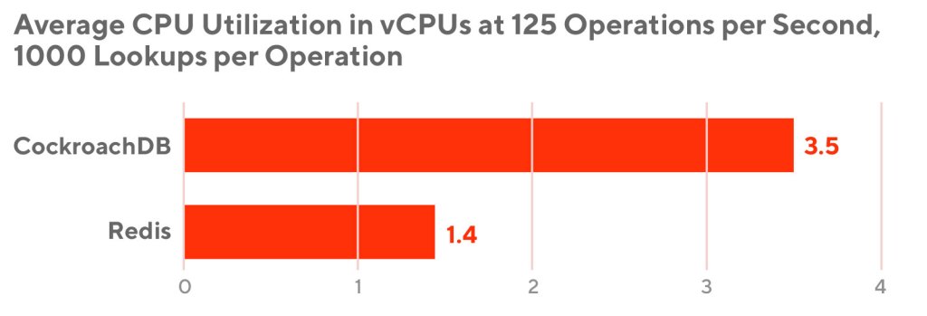
As we can see, even though CockroachDB would provide a much higher storage capacity per node, we still need greater than twice the number of nodes than Redis to support the required throughput. It turns out that the estimated number of nodes needed to support millions of reads per second is so large (10,000 operations per second) that storage is no longer the limiting factor. And thus, Redis beats CockroachDB in costs as well because it performs better with CPU utilization.

We established that Redis is better than CockroachDB in both performance and costs for our setup. Next, we will see how we can optimize Redis so that we can reduce costs even more. 

Optimizing Redis to reduce operation costs

As we learned above, to reduce operation costs, we need to work on two fronts, improving CPU utilization and reducing the memory footprint. We will describe how we tackled each one of these below.

Improving compute efficiency using Redis hashes

In our experiments above, we stored features as a flat list of key-value pairs. Redis provides a hash data type designed to store objects such as user with fields such as name, surname. The main benefit here versus a flat list of key-value pairs is two-fold:

• Collocation of an object’s fields in the same Redis node. Continuing on our example of a user object, querying for multiple fields of a user is more efficient when these fields are stored in one node of a Redis cluster as compared to querying when fields are scattered in multiple nodes.

• Smaller number of Redis commands per batch lookup. With Redis hashes, we need just one Redis HMGET command per entity as opposed to multiple GET calls if features of the entity were stored as individual key-value pairs. Reducing the number of Redis commands sent not only improves read performance but also improves CPU efficiency of Redis per batch lookup.

To exploit Redis hashes, we changed our storage pattern from a flat list of key-value pairs to a Redis hash per entity. That is,

From:

SET feature_name_for_entity_id feature_value

To:

HSET entity_id feature_name feature_value

And our batch reads per entity now look like:

HMGET entity_id feature_name1 feature_name2 ...

The downside, however, of using Redis hashes is that expiration times (TTLs) can only be set at the top level key, i.e. entity_id, and not on the nested hash fields, i.e. feature_name1, etc. With no TTLs, the nested hash fields won’t be evicted automatically and have to be explicitly removed if required.

We will elaborate in the results section how this redesign dramatically reduces not just compute efficiency but also memory footprint.

Reducing memory footprint using string hashing, binary serialization, and compression

To reduce the memory footprint, we will target the feature_name and feature_value portion of our design and try to minimize the number of bytes needed to store a feature. Reducing bytes per feature is not only important for determining overall storage needs but also to maintain Redis hash efficiency, as they work best when hashmap sizes are small. Here, we will discuss why and how we used xxHash string hashing on feature names and protocol buffers and Snappy compression on feature values to cut the size of feature data in Redis. 

Converting feature names to integers using xxHash for efficiency and compactness

For better human readability, we were initially storing feature names using verbose strings such as daf_cs_p6m_consumer2vec_emb. Although the verbose strings work great for communication across teams and facilitating loose coupling across systems referencing these features as a string, it is inefficient for storage. Feature names represented as strings are 27 bytes long whereas a 32 bit integer is, well, 32 bits. Maintaining an enum or keeping a map of feature names to integers is not only extra bookkeeping but also requires all involved systems to be in sync on these mappings.

Using a string hash function guarantees that we will have consistent references of a feature name as integer across all systems. Using a non-cryptographic hash function will ensure we incur minimal computational overheads to compute the hash. Thus, we chose xxHash. We used 32 bit hashing to minimize the probability of hash collisions. This approach can be visualized by changing our HSET command above from:

HSET entity_id feature_name feature_value

to:

HSET entity_id XXHash32(feature_name) feature_value

Binary serialization of compound data types using protobufs

As we discussed before, features such as vector embeddings or integer lists are DoorDash’s compound data types. For the purpose of storage, a vector embedding is a list of float values. To serialize compound data types, we used bytes returned via protocol buffer format. Serializing simple float values to binary did not yield any gains because a significant number of our feature values are zeros. Since we expect a skewed presence of zero values for our float-based features in the future, we chose string as a format of representation because zeros are best represented via strings as a single byte, ‘0’. Putting it all together, serializing compound types with protobufs and floats as strings became our custom serialization approach to maximize storage efficiency.

Compressing integer lists using Snappy

Compressing lists is an additional post-processing step that we apply on top of conversion to the protobufs mentioned above for furthering our size reduction efforts. When choosing a compression algorithm, we needed a high compression ratio and lower deserialization overheads. We chose Snappy for its large compression ratio and low deserialization overheads. 

Additionally, we observed that not all compound data types should be compressed. Embeddings have less compressibility due to being inherently high in entropy (noted in the research paper Relationship Between Entropy and Test Data Compression) and do not show any gains with compression. We have summarized the combination of binary serialization and compression approaches in Table 3 to reflect our overall strategy by feature type.

Feature Type	Redis Value
Float	String form(better than binary serialization when floats are mostly zeros)
Embedding	Byte encoding of Embedding protobuf
Int List	Snappy Compressed byte encoding of Int List as a protobuf(compression is effective when values repeat in int list)

Evaluation and results

Below we report results obtained after pursuing the optimizations reported above. We will dissect the recommendations individually to give a sense of how much incremental impact we get from each one of these. We will show that restructuring flat key-value pairs to hashes has the greatest impact on both CPU efficiency and memory footprint.  Finally, we will demonstrate how all these optimizations sum up to increase the capacity of our production cluster by nearly three times..

Redis with hashes improves CPU efficiency and read latency

We extended our benchmark report to add Redis redesigned with hashes to study the effect it has on read performance and CPU efficiency. We created a new workload which will still perform 1,000 lookups per operation but will break these lookups into 100 Redis key lookups and 10 Redis hash field lookups per key.  Also, for the sake of fair comparison with CockroachDB, we reoriented its schema to make value to be JSONB type and used YCSB’s postgrenosql client to do 100 key lookups and 10 JSONB field lookups per key. 

Note: CockroachDB JSONB fields will not be sustainable for production as JSONB fields are recommended to be under 1MB. Redis hashes, on the other hand, can hold four billion key-value pairs.

CockroachDB NoSQL table schema:

CREATE TABLE table (key varchar primary key, value jsonb)

SQL clause for CockroachDB NoSQL variant:

SELECT key, value ->> field1, value ->> field2, …, value ->> field10
FROM table
WHERE key in (key1, key2, .. key100)

As Table 4 shows, read latency for Redis with hashes has a consistent improvement across both read-heavy and read-only workloads.

Redis hashes and compression combine to reduce cluster memory

As we mentioned earlier, Redis hashes not only improve CPU efficiency but also reduce the overall memory footprint. To demonstrate this, we took a sample of one million records from our table with stratified sampling across different types of features. Table 5 shows that Redis hashes amount to much larger gains as compared to gains with compression.

Setup	In-memory allocation for 1M records	Time to upload 1M records	DB latency per 1000 lookups	Deserialization of 1000 lookup values
Flat key-value pairs	700.2MiB	50s	6ms	2ms
Using Redis hashes	422MiB	49s	2.5ms	2ms
LZ4 compressionon list features in Redis hash	397.5MiB	33s	2.1ms	6.5ms
Snappy compression on list features in Redis hash	377MiB	44s	2.5ms	1.9ms

String hashing on Redis key names saves another 15% on cluster memory

With string hashing, we saw Redis in-cluster memory drop to 280MB when applied at the top of LZ4 compression for the same sample of one million records we used above. There was no additional computational overhead observed. 

For the sample of one million records, we were able to get down to 280MB from 700MB. When we applied the above optimizations to production Redis clusters, we observed perfectly analogous gains, a two and half times reduction, reflecting the viability of our local tests. However, we did not get completely analogous gains on CPU efficiency because CPU spent on requests in production depends on distribution of the keys queried and not the keys stored. YCSB doesn’t allow setting a custom distribution on keys queried and thus was not part of our benchmark setup. 

Overall impact on DoorDash’s production Redis cluster

When implementing all the said optimizations, launching and comparing it with the Redis cluster we had before, we saw memory overall reduce from 298 GB RAM to 112 GB RAM per billion features. Average CPU utilization across all nodes dropped from 208 vCPUs to 72 vCPUs per 10 million reads-per-second, as illustrated in Figure 3, below. 

Furthermore, we saw our read latency from Redis improve by 40% for our characteristic model prediction requests, which typically involve about 1,000 feature lookups per request. Overall latency for our feature store interface, including reads from Redis and deserialization, was improved by about 15%, as illustrated in Figure 4, below.

Conclusion

A large scale feature store used under the requirements for high throughput, batch random reads, and the constraints of low latency is best implemented using Redis. We illustrated using benchmarking on a list of candidate key-value stores that Redis is not only highly performant but is also the most cost-efficient solution under these circumstances. 

We used DoorDash’s feature data and its characteristics to come up with a curated set of optimizations to further improve upon cost efficiency of its feature store. These optimizations exploited Redis hashes to improve CPU efficiency and memory footprint. We also learned that string hashing can effect sizable reductions on the memory requirements. We showed how compression is an effective approach to make compact representation of complex features. While compression sounds counterintuitive when we talk about speed, in specific cases it helps by reducing the size of the payload.

We believe the techniques mentioned for benchmarking can greatly help teams in any domain understand the performance and limitations of their key-value stores. For teams working with large scale Redis deployments, our optimization techniques can provide analogous returns depending on the nature of data in operation. 

Future Work

Continuing upon the performance and efficiency of our feature store, we will investigate exploiting the sparse nature of our feature data to achieve a more compact representation of our feature data.

Acknowledgements

Many thanks to Kornel Csernai and Swaroop Chitlur for their guidance, support, and reviews throughout the course of this work. Thanks to Jimmy Zhou in identifying the need to look into Redis bottlenecks and pushing us in driving this project through. And thanks to the mentorship of Hien Luu and Param Reddy on making this and many other projects for our ML Platform a success. Also, this blog wouldn’t have been possible without the editorial efforts of Ezra Berger and Wayne Cunningham.