
In the fast-paced world of food delivery, accurate estimated time of arrival, or ETA, predictions are not just a convenience; they're a critical component of operational efficiency and customer satisfaction. At DoorDash, where we handle over 2 billion orders annually, the challenge of providing accurate ETAs is both complex and essential.
Traditionally, we have relied on tree-based models to forecast delivery times. While these models produced reasonable forecasts, they also were limited in their ability to capture the intricate patterns and nuances inherent in our vast and varied delivery network. As our operations scaled and customer expectations evolved, we recognized the need for a more sophisticated approach.
Enter our latest innovation: A cutting-edge ETA prediction model that leverages advanced machine learning techniques to dramatically improve accuracy. By leveraging an Multi-Layer-Perceptron-gated mixture of experts, or MLP-gated MoE, architecture with three specialized encoders — DeepNet, CrossNet, and transformer — we created a model that can adapt to diverse scenarios and learn complex relationships from embeddings and time series data to capture temporal and spatial patterns. Additionally, our new approach also incorporates multitask learning to allow the model to simultaneously predict multiple related outcomes. Finally, we explored novel probabilistic modeling approaches to expand the model’s capability to accurately quantify the uncertainty of the ETA forecasts.
The result? A remarkable 20% relative improvement in ETA accuracy. This leap forward not only enhances our operational efficiency but also significantly boosts the reliability of the ETAs we provide to our customers.
We have an earlier blog post that goes deeper into the business context and the problem space. In this post, we dive deep into the technical details of our new ETA prediction system and illustrate how each component contributes to its success as well as how this new approach impacts our business and user experience.
What is ETA?
Before jumping into the modeling details, let’s take a look at the time of arrival we are trying to estimate.
Time of Arrival = Order Creation Time + Delivery Duration
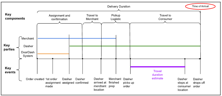
Figure 1: These are the various steps of delivery, broken down by stage and parties involved
In Figure 1 above, we can see the components that contribute to delivery duration for a regular order. In even the most straightforward cases, there are at least three key parties: merchant, Dasher and DoorDash system. We also can break down delivery duration into several stages: Dasher assignment and confirmation, travel to merchant, pickup logistics, and travel to consumer. Given the various parties and stages, a change in any one of them can introduce variation in actual delivery time, which requires us to use more capable tools to tackle the prediction.
Embeddings and time series features
Advanced feature engineering makes up a crucial component of our improved ETA prediction model. Although we kept a number of existing features, we also leveraged neural network embeddings to represent categorical or bucketized continuous inputs, and incorporated time series features, significantly enhancing our model's ability to capture complex patterns and relationships.
Embeddings for rich feature representation
We observed strong predictive signals in categorical features with high cardinality. For example, there are many stores on the DoorDash platform and some — for store-specific reasons such as cuisine type, store popularity, or efficiency — have a longer food preparation time than others. Also, restaurant traffic patterns change over the course of a day with meal times drawing the largest crowds and subsequently increasing delivery duration.
We used feature encoding methods to capture category-based patterns such as one-hot encoding, target encoding, and label encoding. However, one-hot encoding cannot scale efficiently for categorical features with high cardinality because of the curse of dimensionality; other encoding methods are not adequate to capture each category’s patterns because manual effort is required, often causing the loss of semantic relationships. For example, it’s hard for the ETA model to learn similarities between two fast food restaurants when they are compared with other types of restaurants.
To resolve these problems, we introduced embedding into the ETA prediction model. With embeddings, we can convert sparse variables into dense vector representations. At the same time, we improve the generalizability and balance the model's focus on sparse features versus dense features by quantizing and embedding key numerical features. This approach provides such benefits as:
- Dimensionality flexibility: The embedding size is based on the importance of each categorical feature to ETA prediction instead of its cardinality, as would be done with one-hot encoding. We tend to use smaller embedding sizes to avoid overfitting and to reduce model size.
- Capturing category-specific patterns: Embeddings can capture intrinsic patterns and similarities between categories, allowing the model to understand relationships from multiple dimensions; target encoding, frequency encoding, and label encoding can only capture limited amounts of information.
- Improved generalization: The representation of quantized dense features allows the model to generalize better to unseen or rare values. For example, some dense feature values can be extremely high. These outliers can be less impactful during inference because they likely will be capped by the bucket they fall into; the bucket will have plenty of training data to find its embedding representation.
- Flexibility in feature combination: Embedded features can easily be combined with other numerical inputs, allowing for more complex interactions.
- Reusability in other models: The trained embedding can be extracted out and used as input for other models. In this way, the knowledge learned by one ETA model can easily be transferred to other tasks.
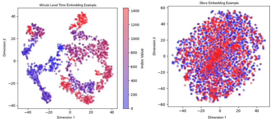
Our ETA model learns the embeddings for categorical features such as time buckets, pick-up and drop-off locations in various granularities, store type, item taxonomies, and assignment segments. Figure 2 below shows examples of time embedding and store embedding. In the time embedding example, blue dots represent earlier in the day while red dots are for later. Closer minutes cluster together; In some cases, such as when the end of one day is closely followed by the start of the next day’s business, both red and blue dots can be found together. In the store embedding example, blue dots represent the stores that use a more standardized order system while red dots refer to an order system used by smaller merchants. We observe that there are multiple clusters of red dots, which may be a sign that this order system more strongly impacts store efficiency, which has a bearing on delivery time. These embeddings and other parameters are input into the DeepNet and CrossNet encoders to capture both deep non-linear patterns and explicit feature interactions.
There also are other important numerical features, such as travel duration and subtotal of order cart. We transform these continuous features into discrete values via bucketization. This makes our model more robust to outliers because the buckets cap outliers, improving the model’s generalization. It also allows for learning complex patterns within each bucket and better captures non-linear relationships. Meanwhile, the original feature values are not discarded, but are also fed to the DeepNet encoder so that we don’t lose precision due to discretization, providing flexibility in handling different types of patterns.
Incorporating time series features
Our ETA model performs well when the overall market dynamic is normal. When there is a shift toward Dasher undersupply, either regionally or in a sub-region, the model’s performance drops. This is caused by old features capturing only high-level supply/demand conditions and being volatile to fluctuations. Both make the feature noisier, which makes it harder for our model to learn the pattern well.
We observed a strong correlation between earlier orders and the later orders in a small time window. For example, if an area is already suffering from an undersupply of Dashers, orders placed in the next quick time window are added to the queue, which leads to cumulative undersupply effects. To take advantage of this temporal nature of delivery ETAs, incorporating time series features has been crucial in responding faster to dynamic changes in the system.
To convey this real-time trend information to our model, we collect time series signals on a minute-level frequency, such as the average order volume per minute over the past 30 minutes. Compared with the average value over the past 30 minutes, this time series conveys richer information about market dynamics. Because this type of feature can be sparse if the time bucket is small, we use the aggregated value of the five-minute bucket and then add learnable positional embedding. With the transformer encoder learning representation from the sequential data, the ETA model learns a representation for the contextual snapshot of the market dynamic in the past time window.
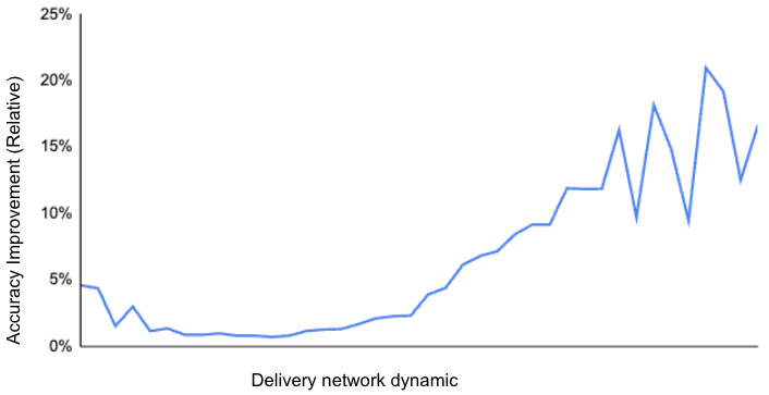
We compared the model performance with and without the time series features and found that the performance improvement can be attributed primarily to better responsiveness to various market conditions, especially when there is significant undersupply of Dashers, as shown in Figure 3 by the higher network dynamic. This suggests that our model now has adapted better to changing conditions over time, such as evolving order patterns or a shifting network dynamic.
While this approach offers significant advantages, it comes at a price: increased computational complexity. The feature engineering method and the transformer encoder both contribute to heavier computational loads during training and inference. Thanks to our Machine Learning Platform team’s strong support, this is successfully productionized and benefiting our consumers with better-quality ETA predictions.
Understanding MLP-gated MoE architecture
We faced several challenges when improving the accuracy of our tree-based ETA model. The model’s predictions had less variance than the ground truth, indicating limited expressiveness, which hindered our ability to capture the full complexity and variability of the target variable, especially in the long tail.
Additionally, the curse of dimensionality made it difficult to identify meaningful splits, leading to overfitting and underfitting, particularly with sparse features. Error analysis suggested that incorporating feature interactions and temporal dependencies could help, but manually creating these interactions was unscalable and noise in the data worsened the dimensionality issue, making it hard to extract useful patterns.
At the heart of our improved ETA prediction model lies an MLP-gated MoE architecture that improves the model’s expressiveness and learns various types of information automatically. This approach allows us to leverage the strengths of different neural network structures, each specializing in capturing specific aspects of the complex relationships within our data. The following sections describe the key components of this architecture.
Parallel encoders
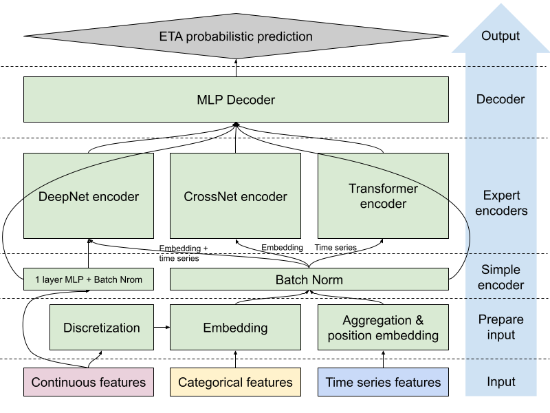
As shown in Figure 4 below, our MLP-gated MoE model employs three parallel encoders, each serving as an expert in processing different aspects of the input data:
- Simple encoder: This one-layer MLP serves two main purposes: convert the input into a fixed dimension that makes adding/dropping features easier and normalize feature values before feeding them to the experts.
- DeepNet encoder: This deep neural network processes inputs through multiple layers, including numerical features, embeddings, and aggregated time series features. It excels at capturing general feature interactions and learning hierarchical representations of the data and is particularly effective at understanding complex, non-linear relationships between various input features.
- CrossNet encoder: Inspired by DCN v2 from recommendation models, CrossNet encoder defines learnable crossing parameters per layer as low-rank matrices and incorporates a mixture of experts with a gating mechanism that adaptively combines the learned interactions based on the input. In the ETA prediction, the input of this expert includes all embeddings of categorical features and bucketized numerical features. The CrossNet encoder is designed to effectively model the complexities and interdependencies between temporal/spatial/order features. At the same time, the depth and the complexity of the interactions are constrained by the number of cross layers and the rank of matrices, leading to both regulatory effect and better computational efficiency.
- Transformer encoder: Leveraging the power of self-attention mechanisms, the transformer encoder focuses on modeling sequential dependencies and relationships. The input of this expert only includes the time series feature, which is a sequence of signals. If fed only into the DeepNet encoder, our ETA model would capture non-sequential, hierarchical patterns and complex feature interactions but may ignore sequence order information. That’s where the transformer encoder comes in; it can learn long-range dependencies and contextual relationships within sequences using self-attention. Temporal dependencies mean that this sequential understanding is helpful for ETA predictions. The ETA model can respond faster to dynamic change if it is exposed to the temporal relationships of volume, delivery cycle, and supply/demand.
Combining expert opinions
Each of these encoders processes different input features, leading to comprehensive learning around various aspects of the information. We bring together the expert opinions from each encoder into a single, rich representation, which is then fed into a multi-layer perceptron to translate the combined insights into an ETA prediction. This simplified architecture differs from a traditional MoE in that it doesn't use a separate gating network to dynamically weight the contributions of each expert. Instead, based on the learned representation from the time series feature, the MLP decoder is aware of the dynamics, so the trained MLP decoder can effectively combine and utilize the outputs from all encoders simultaneously based on different situations. We dropped the explicit gating network because it doesn’t provide meaningful incremental performance improvements in ETA predictions.
This MLP-gated MoE architecture allows us to harness the strengths of different neural network structures while maintaining a manageable level of complexity. One of the key advantages of this approach lies in its extensibility. This allows easy incorporation of additional encoders or other model components without needing to redesign the gating mechanism. The architecture can be adapted to handle the integration of new features, making the model more versatile in responding to changing requirements or data patterns.
As we continue to explore these avenues, further research into optimizing the integration of different encoders — whether through more sophisticated MLP designs or novel gating mechanisms — could unlock even greater performance gains. Ultimately, this approach positions us to stay ahead of the curve in model development, creating a framework that is not only powerful today but also built for tomorrow’s innovations.
Estimating and communicating uncertainty in ETA predictions
In the world of food delivery, providing accurate ETAs is crucial. Equally important, however, is our ability to quantify and communicate the uncertainty associated with these predictions. This is where our probabilistic approach to ETA prediction comes into play, adding a new dimension of reliability to our estimates.
Probabilistic predictions
Traditional ETA models often provide a single-point estimate, which can be misleading in highly variable environments like food delivery. Our approach goes beyond this by implementing a probabilistic base layer for estimating uncertainty in our predictions.
We have explored four approaches to determine the uncertainty about a single prediction:
- Point estimate: We discovered that there’s a consistent trend between the point estimation and the variance of ground truth. Based on this observation, we created a formula to translate point estimate to uncertainty.
- Sampling: For each prediction, we run the inference multiple times, randomly disabling select sets of nodes; we then use the distribution formed by all the inference results as the final prediction.
- Parametric distribution: We assume which distribution family should hold the ground truth and then let the model predict the parameters.
- Non-parametric distribution: We make no assumptions about the distribution itself, instead assuming the range in which the ground truth might fall. The possible range is segmented into multiple buckets and then the model predicts the probability for each bucket. We can get a good estimate of the probability density function by tuning the granularity or smoothing techniques.
By incorporating this probabilistic base layer, our model doesn't just predict a single ETA value, but rather a distribution of possible arrival times. This distribution provides valuable information about the uncertainty associated with each prediction.
Challenges of learning a Weibull distribution
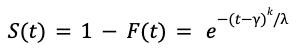
In previous blog posts in 2021 and 2022, we reported strong evidence that the food delivery time follows a long-tail distribution that cannot be modeled by Gaussian or exponential distributions. To capture the long-tail nature and accurately predict the uncertainty for each delivery, we chose to model the food delivery time via the Weibull distribution, whose probability distribution function takes the form:

The parameters 𝑘, 𝝀, 𝛾 are called the shape, scale, and location of the Weibull distribution and they specify the distribution’s tail shape, width, and minimum. The machine learning task is to train AI models to predict these parameters 𝑘, 𝝀, 𝛾 as functions of the input features 𝑋.
When we trained the AI model to maximize the log-likelihood under Weibull distribution, we found that the model sometimes makes unreasonable predictions. For instance, the model may predict a negative location 𝛾 < 𝑂, which means a non-zero chance that the food is delivered within one minute of placing the order, which is impossible in reality. The key challenge is that the parameters 𝑘, 𝝀, 𝛾 appear in the log-likelihood function in highly nonlinear forms

and it is likely that the model overfits the observed data.
Interval regression
Because using the log-likelihood loss function did not lead to accurate predictions, we needed to modify the loss function to make it easier to learn the Weibull distribution parameters. After multiple trials, we proposed an innovative approach to use the survival function 𝑆(𝑡), defined as:
We further leveraged the log-log transform of the survival function, which takes a much simpler functional form:

Using this as the loss function, we used simple least squares to fit the Weibull distribution parameters 𝑘, 𝝀, 𝛾.
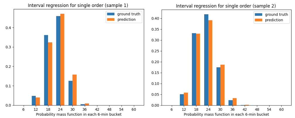
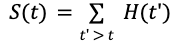
Finally, we needed to derive the survival function 𝑆(𝑡) from data. Interval regression provides a solution, grouping the deliveries with similar input features 𝑋 and plotting a histogram of the food delivery time 𝐻(𝑡) where the length of each bucket is six minutes, shown in Figure 5 below.
The survival function at each time t is derived by simply summing the histogram values for 𝑡' > 𝑡:
A simulation study
We validated the prediction accuracy of the interval regression approach via a simulation study. For each delivery with input features 𝑋, we used fixed functions to generate the ground truth parameters
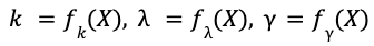
The AI models must learn these functions 𝑓𝑘, 𝑓𝜆, 𝑓𝛾. Given each set of input features 𝑋, we simulate 1 million observations by drawing random samples from the Weibull distribution with these parameters 𝑘, 𝝀, 𝛾. This forms the training and validation datasets.
Next, we use the interval regression approach and train a multi-head neural network to simultaneously learn the functions 𝑓𝑘, 𝑓𝜆, 𝑓𝛾. We compare the predicted parameters against their ground truth values and measure the accuracy of the distribution predictions.
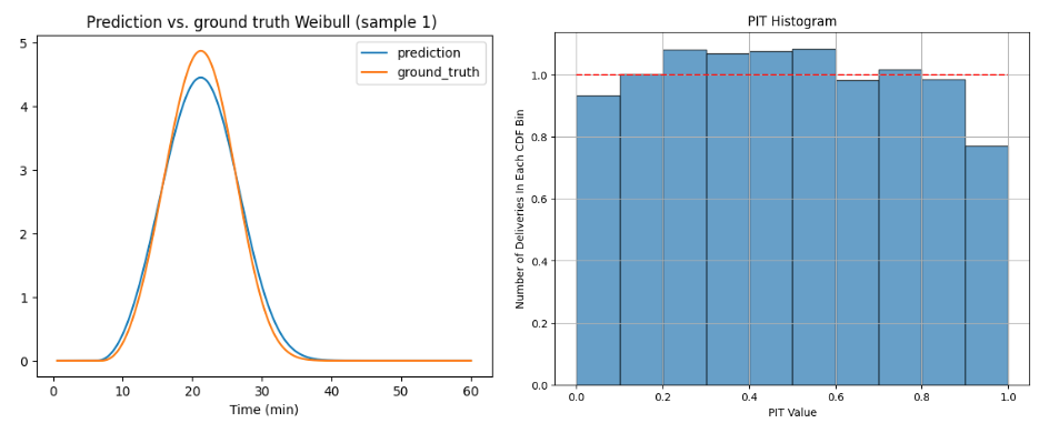
We found that our interval regression approach greatly reduced the problem of overfitting and predicted more accurate values of the Weibull parameters. As shown in Figure 6, the ground truth parameters are 𝑘 = 3.37, 𝜆 = 0.27, 𝛾 = 0.11 while their predicted values are 𝑘 = 3.22, 𝜆 = 0.28, 𝛾 = 0.10. The model calibration, measured by PIT histogram (Figure 6), is also greatly improved as a result.
Interval regression allows us to simultaneously learn the shape, scale, and location parameters of the Weibull distribution with high accuracy. Our next step is to apply the interval regression approach to real delivery data. We can then leverage the predicted probability distributions to give customers the most accurate possible ETAs for food delivery while reliably estimating the uncertainty in these ETA predictions.
We are still exploring the best way to predict ETA uncertainties so that we can continue to improve our service’s accuracy and transparency. Understanding ETA uncertainty also enables more efficient allocation of Dashers and better route planning. This probabilistic approach represents a significant step forward in our mission to provide the best possible delivery experience for our customers and partners.
Leveraging multitask learning for diverse ETA scenarios
The consumer journey of placing a delivery order comes in two stages: explore stage and checkout stage, as shown in Figure 7 below. The explore stage is when consumers are browsing through stores without adding any items to their shopping cart yet. At this stage, we can only access features related to store or consumer historical behavior. In the checkout stage, consumers have built an order cart, so we also access item information. We used models trained individually to support these two stages but we found that this can lead to estimation inconsistencies. Big differences surprise consumers in negative ways that undermine their trust in our estimates. Our initial attempt to mitigate this has been to enforce an adjustment on the later stage based on former estimations. This adjustment improved consistency but lowered accuracy. In the later stage, the estimation is usually more accurate because of better data availability. This adjustment is based on estimation from former stages, which introduces reduced accuracy. To address the inconsistency without hurting accuracy, we've implemented a multitask learning approach to develop our ETA prediction model. This strategy allows us to handle different ETA scenarios together, leading to more consistent and efficient predictions. Let's dive into the specifics of our approach and its benefits.

Shared vs. task-specific
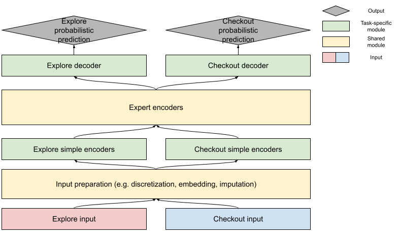
Coming up with an ETA prediction involves developing both explore and checkout probabilistic predictions. These two tasks have much in common, with labels -- actual delivery duration — shared between both. In the majority of samples, the store- and consumer-related feature values are very close. So we can expect the learned relationship between these features and labels to be similar. Considering the commonalities, it is also reasonable to share parameters representing the relationship between features and labels. But the availability of order information is different; for some real-time information, the checkout stage’s feature value distribution can be different and usually has higher correlation with the label. Because of these differences, task-specific modules handle the input difference and convert the final encoded representation into the prediction. Figure 8 shows our training design to balance the task-specific accuracy and knowledge sharing:
Co-training vs. sequential training
We began this journey with a critical decision between co-training or sequential training. Co-training, which involves training all tasks simultaneously using a shared model architecture, initially seemed attractive because of its efficient training time and use of computational resources. It also offered the potential for real-time knowledge sharing between tasks. In the end, however, we observed significant degradation in accuracy in individual tasks, likely caused by interference between tasks.
We turned instead to sequential training, where tasks are trained one after another, freezing the parameters learned during previous tasks and training the task-specific parameters for later efforts. Despite being more time-consuming, this approach proved superior for ETA prediction. By isolating the training process for each task, we were able to reduce noise from other tasks and better fine-tune task-specific parameters. Crucially, this method facilitated effective learning transfer by sharing parameters between tasks while minimizing interference.
The sequential training approach that we implemented begins with training our model on checkout tasks. Once this task is well-learned, we freeze all checkout-related parameters and move on to train the light-weighted explore-specific parameters. Because the checkout task has higher priority and richer information, it’s better to train the majority of parameters, such as embeddings and expert encoders, on it. Accuracy improvements in the explore task also show the successful knowledge transfer.
Benefits of multitask training
The benefits of this multitask learning approach have been substantial and far-reaching. First and foremost, we've achieved remarkable consistency improvement in ETA predictions across different stages without sacrificing accuracy. Moreover, despite the sequential nature of our training process, this approach has proved more efficient than training separate models for each stage. The shared components provide a warm start for other scenarios, simplifying development and reducing velocity, a crucial consideration at our scale of operations.
Perhaps most excitingly, we've observed significant learning transfer between stages, improving explore task performance through fine-tuning the checkout task model. This opens the possibility of transferring learned patterns to even more tasks, for example using the store embedding for other downstream business problems.
Multitask learning has been a cornerstone in improving our ETA accuracy. By leveraging the strengths of sequential training and the benefits of multitask learning, we've created a more robust, efficient, and accurate ETA prediction system. As we continue to refine and expand our multitask learning approach, we're excited about its potential to further enhance our ETA predictions, ultimately leading to better customer experiences, more efficient partner operations, and smoother Dasher deliveries.
Charting the future of delivery time estimation
As we conclude our deep dive into DoorDash's latest advancements in ETA prediction, it's clear that our journey toward more accurate and reliable delivery times has yielded impressive results. The remarkable 20% relative improvement in ETA accuracy stands as a testament to our team's innovative approach and relentless pursuit of excellence. We enhanced precision for both large and small orders, long- and short-distance deliveries, and during both peak and off-peak hours. This advancement directly improves our customer experience by minimizing unexpected delays and preventing premature arrivals. As a result, our customers can now place greater trust in our estimated delivery times, allowing them to plan their schedules with increased confidence.
This significant leap forward is the culmination of several advanced techniques. Our simplified MoE architecture, with its parallel encoders and novel combination approach, has proven adept at handling the diverse scenarios inherent in food delivery. Advanced feature engineering, which leverages embeddings and time series data, has enhanced the model's ability to capture nuanced patterns and temporal dependencies. The multitask learning approach and its sequential training have improved consistency across various ETA scenarios while facilitating valuable knowledge transfer between tasks. Finally, the introduction of probabilistic predictions expands our model’s potential by enriching predictions with more probabilistic context.
These advancements have had a profound impact on DoorDash's operations, leading to more efficient logistics, improved customer satisfaction, and a more seamless experience for our entire ecosystem of customers, Dashers, and merchants.
Nonetheless, we recognize that the pursuit of perfect ETAs is an ongoing journey. Looking ahead, we're excited to explore new frontiers in delivery time estimation. Our commitment to innovation remains unwavering. We believe that by constantly improving our ETA predictions, we can create an even better experience for everyone in the DoorDash community. We hope this blog post has provided valuable insights into the complex world of ETA prediction and the innovative solutions we're implementing at DoorDash.
Acknowledgments
Special thanks to Vasundhara Rawat, Shawn Liang, Bin Rong, Bo Li, Minh Nguyen, Kosha Shah, Jie Qin, Bowen Dan, Steve Guo, Songze Li, Vasily Vlasov, Julian Panero, and Lewis Warne for making the ETA model improvements possible.